MSc-FinalExam
The Final Chapter of Story
Advanced Software Technology
Software development workflows and methodologies
Software Development Models define the process of building software. They range from rigid plan-driven (Waterfall, V-model) to flexible iterative (Agile, Scrum). The key trade-off is predictability vs adaptability. Old models treat software like manufacturing (build once, replicate), but real software is knowledge creation — requirements change, technology shifts. This is why Agile won: it embraces change instead of fighting it.
cowboy coding
Cowboy Coding means writing code without any process: no design docs, no version control, no tests. Devs just “hack it until it works.”
Key traits: Ad-hoc testing (click around, call it done), fix-on-the-fly (patch production directly), cowboy deployment (FTP files, git pull on prod).
Why it’s deadly: Truck Factor = 1 (only one dev understands the spaghetti code), technical debt explodes (fixing bug A creates bugs B, C, D), modification cost goes exponential over time.
When it works: Solo prototyping for 2 weeks. Never for production teams.
waterfall
Waterfall Model (Royce, 1970) = Requirements → Design → Implementation → Verification → Maintenance. Each phase must 100% complete before the next starts. Phase gates with sign-offs at every stage.
Pros: Highly predictable (cost, schedule known upfront), good for deterministic systems (banking, aerospace firmware).
Cons: Feedback loop is months/years — user sees working software only at the end. Change cost is 10-100x in later phases. Completely wrong for startups where requirements are unknown.
Why it fails in software: Software is not a car factory — copying costs $0, requirements are subjective, change is cheap with good architecture.
agile
Agile Manifesto (2001): Individuals & interactions > processes & tools; Working software > comprehensive docs; Customer collaboration > contract negotiation; Responding to change > following a plan.
Key practices: Self-organizing teams (Two-Pizza: 5-9 people, cross-functional), Incremental development (fixed-length iterations, each produces potentially shippable increment).
Four ceremonies: Sprint Planning (pick backlog items) → Daily Standup (15 min, 3 questions: what I did, what I’ll do, what blocks me) → Sprint Review (demo real software) → Retrospective (what went well, what to improve).
Watch out: “Flaccid Agile” — random standups with no discipline is NOT agile. Real agile demands fixed sprints, a Definition of Done, and a reserve of 15-20% of each cycle for refactoring & automation tests.
TDD
Test-Driven Development (TDD) = Red-Green-Refactor loop:
- Red: Write a failing test first (it forces you to think about requirements before code)
- Green: Write the simplest possible code to pass (even hardcoding)
- Refactor: Clean up code with confidence — tests stay green
Why it works: Tests force you to understand what “done” means before coding. TDD naturally produces decoupled, modular code. Gives team courage to refactor anytime.
Key insight: The test is not a verification step — it’s a design tool. It shapes your architecture from the start.
Pair it with: Pair Programming (Driver writes tests + code, Navigator watches strategy). Costs ~15% overhead but yields 80%+ bug reduction.
scrum
https://aloen.to/Program/Theory/%E8%BD%AF%E4%BB%B6%E6%8A%80%E6%9C%AF/#Scrum
Scrum is a specific Agile framework with fixed Sprints (1-4 weeks, typically 2). The time-box is inviolable — unfinished work goes back to the Backlog, never extend the sprint. No changes allowed mid-sprint.
Three roles: Product Owner (decides what to build, prioritizes Backlog), Scrum Master (servant leader: removes blockers, enforces process), Development Team (self-organizing, decides how).
Key artifacts: Product Backlog (ordered list of everything needed) → Sprint Backlog (tasks committed for this sprint) → Increment (potentially shippable product at sprint end).
The Scrum Master is NOT a project manager — they shield the team from external interruptions, clear roadblocks (broken CI, missing environments), and coach the team in retrospectives.
kanban
Kanban (from Toyota, 1940s) is a pull system — downstream pulls work when ready, upstream doesn’t produce unless asked. Core tool: a visual board with columns (Backlog → Selected → In Dev → QA → Done). Anyone can see in 3 seconds: what the team is doing, what’s blocked, who’s idle.
Soul of Kanban: WIP (Work in Progress) Limits. Each column has a hard limit (e.g., “In Dev” max=3). Little’s Law: Cycle Time = WIP / Throughput. More WIP = longer queues. When a column is blocked, devs must swarm to clear the bottleneck — “Stop Starting, Start Finishing.”
7 Wastes eliminated: Partially done work, over-engineering, extra steps, task switching, waiting, motion, defects.
Kanban vs Scrum: Kanban is continuous flow (no fixed sprints), Scrum is time-boxed iterations. Kanban is better for ops/maintenance, Scrum for product development.
User eXperience
what it is
User Experience (UX) is not just “making it pretty.” It’s about how a person feels when interacting with a product. The golden rule: “Don’t make me think” — good UX is self-explanatory. Users should not need instructions or manuals.
Core principle: Reduce cognitive load. Match existing mental models (gear icon = settings, trash can = delete), use familiar patterns. Every extra click, every confusing label adds “cognitive friction” that drives users away.
UX starts before any code is written — with wireframes, user research, and understanding who the user is and what they need.
its main parts
UX has Three Pillars:
Look (Visual Design): Color psychology (blue/green = trust for finance/health, bright colors = dopamine for entertainment). Design Systems enforce consistency in spacing, grids, typography — mathematical order signals professionalism.
Feel (Interaction): Skeleton screens during loading (not blank white) create perception of speed. Animations follow physics (inertia, damping). Delighters — small animations/haptic feedback on completing key actions release dopamine.
Usability: Predictability (user knows what will happen before clicking), Efficiency (minimize clickstream, auto-focus, smart defaults), Accessibility (a11y) — WCAG contrast ≥4.5:1, never rely solely on red/green (use icons+text), full keyboard navigation.
Requirements: use case diagrams
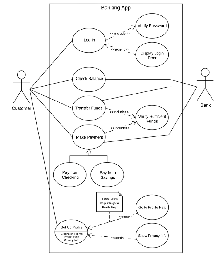
Use Case Diagrams (UML) show who (actors) can do what (use cases) with the system. Actors are stick figures, use cases are ovals, lines connect them. The system boundary is a box. This diagrams the functional requirements at a high level — not how things work, but what the system must do for each user role.
Key insight: A use case describes a goal the user wants to achieve. “Login” is a use case (user wants to prove identity). “Enter password” is NOT a use case (it’s a step toward the goal).
user stories
User Stories are lightweight requirements in the format: As a [role], I want [action] so that [value]. Example: “As a customer, I want to filter products by price so that I can find items in my budget.”
They follow the INVEST criteria: Independent (can be built separately), Negotiable (details can be discussed), Valuable (delivers value to user), Estimable (team can size it), Small (fits in one sprint), Testable (has clear acceptance criteria).
Key insight: User stories replace thick requirement documents. They are placeholders for conversation, not final specs. The team discusses details during sprint planning.
BDD
Behavior-Driven Development (BDD) extends TDD with natural language scenarios using Gherkin syntax:
- Given [initial context]
- When [action happens]
- Then [expected outcome]
Example:
1 | Given a user is logged in |
The “Three Amigos”: Product Manager, Developer, QA write these scenarios together before coding. QA uses them directly as test cases, devs use them with Cucumber/SpecFlow. BDD ensures everyone agrees on what to build before spending time on how to build it.
DevOps
https://aloen.to/Program/Theory/%E8%BD%AF%E4%BB%B6%E6%8A%80%E6%9C%AF/#DevOps
DevOps is a cultural and technical movement to break down silos between Development (who wants to ship fast) and Operations (who wants stability). The classic conflict: “It works on my machine!” → blame game → delayed releases.
CAMS model: Culture (blameless post-mortems, shared responsibility), Automation (CI/CD, Infrastructure as Code), Measurement (DORA metrics: Deployment Frequency, Lead Time, MTTR, Change Failure Rate), Sharing (devs see monitoring, ops see architecture).
DevOps Loop: Code → Build/CI → Test → Package (immutable Docker image) → Release (Blue-Green or Canary deployment) → Configure (IaC) → Monitor & Feedback (logs, APM, alerts) → back to Code.
version control systems
Version Control Systems (VCS) track changes to code over time. Git is the industry standard — a distributed VCS where every developer has a full local repo with complete history.
Three local areas: Working Directory (your current files) → Staging Area (git add) → Local Repository (git commit). Remote sync via git push.
Key concepts: Branches are lightweight pointers to commits. Feature branching isolates new work from main. Trunk-Based Development (TBD) merges to main multiple times per day — feature branches live only hours. Use Feature Toggles (config flags) to merge half-done features without breaking production.
git
Git branching and merging are the heart of parallel development. Two merge types:
- Fast-Forward: No diverging commits, just moves the pointer forward (clean history).
- Three-Way Merge: Creates a merge commit when branches have diverged.
Merge conflicts happen when two branches modify the same line — must be resolved manually. In Trunk-Based Development, conflicts are caught within hours (not days), making them small and easy to fix.
Best practice: Feature branches off main, merge back via Pull Request with Code Review. Every PR should be reviewed by at least one other person before merging.
CI/CD
CI/CD (Continuous Integration / Continuous Deployment) automates the path from code commit to production.
CI: Developers merge to main multiple times per day. An automated pipeline runs: pull code → compile → run all unit tests → code quality scan. 10-minute rule: if the pipeline breaks, the whole team stops to fix it first.
CD: After CI passes, deployment to staging/production is automated. Blue-Green Deployment (two identical clusters, instant switch) or Canary Release (5% → 20% → 50% → 100% traffic ramp-up).
Key benefit: Eliminates “it works on my machine” by running everything in a clean Docker container every time. Failures are caught in minutes, not weeks.
automatic testing
Automatic Testing in the CI pipeline includes multiple levels:
- Unit Tests: Test individual functions/classes. Focus on core business logic (payment, pricing).
- Integration Tests: Test combined modules with real DB/Redis/APIs.
- Code Coverage Gate: e.g., <80% coverage = pipeline rejected.
Pipeline flow: CI server pulls clean Docker container → downloads locked dependencies → compiles → runs static analysis (SonarQube) → runs unit tests → runs integration tests → if ALL pass, creates immutable artifact (Docker image tagged v1.0.4-build28).
The 10-minute rule applies to the full pipeline. If tests take longer, they slow down the entire development cycle.
the three levels of MLOps
MLOps applies DevOps principles to Machine Learning. Three evolution levels:
Level 1 (Manual): Data scientists train models on local machines. Code and model artifacts are shared manually via USB/email. No reproducibility, no tracking. Models are “thrown over the wall” to engineering.
Level 2 (Automated): ML pipelines are automated with CI/CD for training and deployment. Experiment tracking (MLflow, Weights & Biases) logs every run, dataset version, hyperparameter. Models are versioned in a registry. Automated retraining triggers on new data.
Level 3 (Full MLOps): The entire ML lifecycle is automated and monitored. Automated retraining + deployment runs without human intervention. Data and model drift detection (monitoring → alerts → auto-rollback). A/B testing between model versions in production. This is the goal — a self-correcting ML system.
OOP basics
Object-Oriented Programming (OOP) organizes code around objects (data + behavior) rather than functions + data separately. Three core goals: Reusability (classes are Lego bricks), Maintainability (high cohesion, low coupling — changing one class doesn’t ripple everywhere), Team Collaboration (interfaces define contracts between devs).
Key departure from procedural code: OOP bundles state and behavior together. The object is responsible for its own data — no one outside should reach in and manipulate it directly.
classes and objects
Class = a blueprint/template that defines attributes (fields) and capabilities (methods). It describes what an object looks like and what it can do.
Object = a concrete instance of a class, allocated on the heap via new, with its own independent state (the value of its fields) and lifecycle.
Think of a class as a cookie cutter and objects as the cookies. One cookie cutter produces many cookies, each with its own chips (state). The cutter defines the shape, but each cookie exists independently in memory.
class diagram
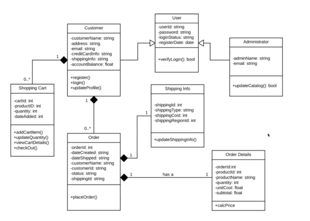
Class Diagrams (UML) visually represent the static structure of a system. Boxes = classes (with name, fields, methods in three compartments). Lines = relationships:
- Arrow (→) = Dependency (temporary use, e.g., method parameter)
- Solid arrow = Association (long-term member field)
- Hollow diamond (◇) = Aggregation (part survives whole)
- Filled diamond (◆) = Composition (part dies with whole)
- Hollow triangle (△) = Inheritance (Is-A)
Class diagrams show what exists and how things relate, not how they run. They are the blueprint before coding begins.
fields
Fields (also called attributes/properties) are the data that an object holds. They represent the state of the object. In well-designed OOP, fields should be private — only the object itself can directly access them.
Access via getters/setters should enforce business rules, not just expose raw data. A setAge(int age) method should validate that age > 0, not just blindly assign. True encapsulation means you can change the internal representation without affecting external code.
methods
Methods define the behavior or operations that an object can perform. They operate on the object’s internal state (its fields) and potentially return results or cause side effects.
Methods implement the interface contract — they define what the object can do. Good methods are cohesive (do one thing well), short (fit on one screen), and named meaningfully (a method called calculateInvoiceTotal() should not also send emails).
Methods are how objects communicate: object A calls object B’s method to request something — Tell, Don’t Ask.
visibility
Visibility (Access Modifiers) control who can see and use fields/methods. From most to least visible:
| UML | Keyword | Who can access |
|---|---|---|
+ |
public |
Any class anywhere (interface contracts) |
# |
protected |
Current class + subclasses only |
~ |
package-private | Same package/namespace only |
- |
private |
Only the current class |
Golden rule: All fields should be private. Make methods public only when they are part of the class’s contract. Protected is for inheritance hooks. Package-private is rarely needed. The more restricted your visibility, the less coupled your code is.
encapsulation
Encapsulation is the bundling of data with methods that operate on that data, and restricting direct access to internal state. It’s NOT just private fields with public getters/setters. A bare setAge(age) { this.age = age; } is NOT encapsulation — it’s just data hiding.
Real encapsulation: Expose business-meaningful methods. Instead of setAge(), provide celebrateBirthday(). Instead of setSalary(), provide applyRaise(percentage). “Tell, Don’t Ask” — tell the object what you want done; don’t reach into its data to figure it out yourself.
Benefit: You can change the internal implementation (e.g., switch from int age to Date birthDate) without breaking any external code.
relationships between classes
Five class relationships, from weakest to strongest coupling:
Dependency (→): Temporary — a class used as a method parameter. Relationship ends when the method returns.
Association (→, solid): Long-term — one class holds a reference to another as a member field. Peers, no ownership.
Aggregation (◇): Whole-part, independent lifetimes. Part survives the whole. E.g.,
UniversityhasList<Professor>— professors exist even if the university closes.Composition (◆): Whole-part, dependent lifetimes. Part dies with whole. E.g.,
CompanyhasList<Department>— departments don’t exist without the company.Inheritance (△): Is-A — subclass inherits all non-private members of parent. Strongest coupling, use sparingly.
inheritance
Inheritance creates an Is-A relationship: class Dog extends Animal. The subclass inherits all non-private fields and methods of the parent. It can then override methods to specialize behavior, or extend by adding new fields/methods.
Problem: Fragile Base Class Problem — modifying the top-level base class can break dozens of subclasses downstream. Inheritance is the tightest coupling in OOP.
Rule of thumb: Prefer composition over inheritance. Inheritance models “what an object IS.” Composition models “what an object HAS.” Most of the time, you want composition — it’s more flexible and less fragile.
Inheritance is appropriate when: There’s a clear taxonomic hierarchy, subclasses truly fulfill the Liskov Substitution Principle, and the hierarchy is stable (rarely changes).
polymorphism
Polymorphism means “many forms” — the same method call behaves differently depending on the actual runtime type of the object. It’s powered by dynamic binding (late binding) : the compiler doesn’t know which implementation will be called; at runtime, the CPU looks up the Virtual Function Table (VTable) in the object header to dispatch to the correct method.
1 | IPaymentStrategy strategy = getPaymentMethod(); // Could be WeChat, AliPay, PayPal |
This + Dependency Inversion (both high and low layers depend on abstractions, not on each other) is the foundation of most design patterns. The high-level CheckoutManager depends only on the IPaymentStrategy interface — the concrete implementation is injected at runtime.
SOLID principles
https://aloen.to/Program/Theory/%E8%BD%AF%E4%BB%B6%E6%8A%80%E6%9C%AF/#SOLID-%E5%8E%9F%E5%88%99
SOLID = 5 principles of OOP design:
Single Responsibility: A class should have only one reason to change. An
Orderclass should notcalculateTax(),saveToMySQL(), andsendConfirmationEmail()— extract DB toOrderRepository, email toNotificationService.Open/Closed: Open for extension, closed for modification. Instead of
if/elsechains for each payment type, use polymorphism — add new types by creating new classes, not editing existing ones.Liskov Substitution: Subclasses must completely replace their base class without breaking logic. A
Squareshould NOT extendRectangle— setting width should not change height.Interface Segregation: Many small, specific interfaces are better than one fat interface.
IWorkerwithwork(),eat(),sleep()forcesRobotWorkerto stub irrelevant methods.Dependency Inversion: High-level modules should not depend on low-level modules. Both should depend on abstractions.
NotificationManagershould depend onIDatabase, notMySQLDatabase.
OOP design patterns
Design Patterns are reusable solutions to common software design problems. They are not code — they are templates for how to structure classes and objects. Three categories: Creational (how objects are created), Structural (how classes are composed), Behavioral (how objects communicate).
Patterns emerged from the collective experience of developers. Using them gives you a shared vocabulary: saying “use a Strategy pattern here” communicates the entire design instantly to any experienced developer.
Strategy
Strategy Pattern defines a family of algorithms, encapsulates each one, and makes them interchangeable. It eliminates if/else or switch chains.
Structure: A Strategy interface (e.g., IRouteStrategy with buildPath()), multiple Concrete Strategies (WalkingStrategy, DrivingStrategy, TransitStrategy), and a Context class that holds a reference to the current strategy.
1 | class Navigator { |
Key benefit: Adding a new algorithm (e.g., BicycleStrategy) requires zero changes to the Navigator class — Open for extension, closed for modification (OCP).
Iterator
Iterator Pattern provides a way to access elements of a collection sequentially without exposing the underlying representation (array, tree, hash map, linked list). Two simple methods:
1 | interface Iterator<T> { |
Why it matters: Client code uses the same while(iterator.hasNext()) { element = iterator.next(); } regardless of whether it’s iterating an array, a binary tree, or a database cursor. The internal complexity is encapsulated behind a simple interface.
This is so fundamental that most languages now have built-in for-each syntax (e.g., for item in collection) which desugars to iterator calls.
Factory
Factory Method delegates object creation to a separate factory class. Instead of new FedExShipping() scattered everywhere, high-level code asks a ShippingFactory to produce the right implementation.
Problem: Direct new creates tight coupling. If you switch from FedEx to SF-Express, you must rewrite every file that contains new FedExShipping().
Solution:
1 | interface IShippingService { void ship(Order o); } |
High-level code only knows IShippingService. The factory decides what to instantiate. This is typically combined with Dependency Injection (Spring, Guice) to auto-wire the correct implementation.
Singleton
Singleton Pattern ensures a class has exactly one instance and provides a global point of access to it. Used for shared resources: configuration manager, database connection pool, logging service.
Implementation: Private constructor + static getInstance() method + static field holding the single instance. Thread-safe initialization (e.g., synchronized or eager initialization) is critical for multi-threaded environments.
Controversy: Many consider Singleton an anti-pattern because it introduces global state, making code harder to test (you can’t mock the singleton in unit tests). Modern alternatives: Dependency Injection manages single instances via IoC containers, giving you testability + the same single-instance behavior.
When to use: Rare. Only when you truly need one instance and it’s acceptable as global state.
Observer
Observer Pattern defines a one-to-many dependency: when one object (the Subject/Publisher) changes state, all its dependents (Observers/Subscribers) are automatically notified. Core mechanism: the Subject maintains a list of Observers and calls each one’s update() method when state changes.
1 | interface IObserver { void update(String event); } |
Push vs Pull: Push model sends all data with the notification (fast but wasteful). Pull model sends only a signal, observers fetch what they need (flexible but more complex).
Use cases: UI event handling (button click → notify listeners), publish-subscribe systems, real-time data feeds.
Decorator
Decorator Pattern dynamically adds responsibilities to an object without modifying its class. It wraps the original object inside a “wrapper” that adds behavior — like Russian nesting dolls.
Problem with inheritance: A simple coffee shop with MilkCoffee, SugarCoffee, MilkAndSugarCoffee → class explosion. Adding caramel creates CaramelCoffee, CaramelMilkCoffee, CaramelSugarCoffee, CaramelMilkSugarCoffee — combinatorial explosion.
Decorator solution:
1 | ICoffee order = new SimpleCoffee(); // $10 |
Each decorator implements the same interface as the original, holds a reference to the wrapped object, and adds its own behavior before/after delegating to the wrapper. This is Open for extension, closed for modification (OCP) in action.
Composite
Composite Pattern treats individual objects (Leaf) and compositions of objects (Composite) uniformly through a common interface. It creates a tree structure where both leaves and branches respond to the same method call.
1 | interface FileSystemComponent { long getSize(); } |
Key insight: The caller doesn’t know (and doesn’t care) whether it’s dealing with a single file or a directory tree. Recursive composition via the same interface makes the code incredibly clean.
Embodied Intelligence
https://aloen.to/AI/EI/Embodied-Intelligence/
Embodied Intelligence (EI) is the study of intelligent systems that have a physical body (embodiment) interacting with the real world. Unlike pure AI (which lives in data), EI must deal with physics, uncertainty, and real-time constraints. Core components: Embedded Systems (the computational + sensing/acting platform), Ethorobotics (animal-inspired robots), Cognitive Robotics (robot minds), Evolutionary Robotics (optimization through evolution), and Biologically-inspired locomotion (how robots move).
Embedded Systems
Main building blocks and their relationship with the environment
An embedded system has three main building blocks forming a mechatronic closed loop:
Sensor: Detects a physical event/change in the environment (light, temperature, pressure) and outputs an electrical signal. Like human eyes/ears/skin.
Computational Unit (Microcontroller/MCU): The “brain” — handles signal processing, decision making, control signal generation, and communication. It’s the cortex that interprets sensor data and commands actuators.
Actuator: Interacts with the environment based on commands. Motors, linear drives, etc. Like human muscles.
The loop: Environment → Sensor → (A/D conversion) → Computation → (D/A conversion) → Actuator → Environment — continuous, real-time information exchange.
Control loops (open/closed)
Open-loop control: Actuate without feedback. The system calculates the required action based on a mathematical model (inverse dynamics) and executes it blindly. Pros: Simple, fast. Cons: Cannot compensate for disturbances (friction, load changes). A robot arm that doesn’t check if it actually reached the target will drift over time.
Closed-loop control: Actuate with feedback. A sensor measures the actual output, compares it to the target (error = target - actual), and adjusts accordingly. The PID controller dominates 90%+ of industrial and robotics control:
$$u(t) = K_p e(t) + K_i \int_0^t e(\tau) d\tau + K_d \frac{de(t)}{dt}$$
- P (Proportional): Reacts to current error. Big error = big force. Alone, causes steady-state error.
- I (Integral): Accumulates past error. Eliminates steady-state error by building up force over time.
- D (Derivative): Predicts future error. Dampens oscillations, acts as a shock absorber.
Key concept: GIGO (Garbage In, Garbage Out) — if the feedback signal is noisy, control will be poor.
Signal Types of signals (based on the time/value quantization)
Signals are classified by how time and amplitude are quantized:
Analog (Continuous time + Continuous amplitude): The real-world signal — infinitely variable in both domains. Microphone output, temperature voltage.
Discrete-time (Sampled): Time is quantized (sampled at intervals like 1ms), but each sample’s amplitude remains continuous. The output of a sample-and-hold circuit.
Discrete-amplitude (Quantized): Time is continuous, but amplitude can only take discrete levels. The output of an ADC before the next time step — rarely exists in isolation.
Digital (Discrete time + Discrete amplitude): Both time and amplitude are quantized. The computer’s world — everything is 0s and 1s, processed in clock cycles.
The fundamental cost: Quantization error — when converting analog to digital, you lose information. An 8-bit ADC divides a 3.3V range into only 256 steps. The lost detail = quantization noise.
Signal preprocessing methods
Signal Conditioning is the manipulation of raw sensor signals to make them usable by the next stage. Key operations:
Amplification: Raw sensor signals are often millivolts — too small for an ADC. Op-amps boost them to 0-5V range.
Filtering: Remove noise that corrupts the signal. Keep the useful information, discard unwanted frequencies.
Converting: Change signal type — voltage to current, differential to single-ended, etc.
Range Matching: The ADC expects 0-3.3V, but the sensor outputs 0-10V. Scale it down (voltage divider) or up.
Isolation: Optical or transformer isolation protects the sensitive MCU from high-voltage spikes on the sensor side (common in industrial motors).
Key metric: Signal-to-Noise Ratio (SNR) = $10 \log_{10}(P_{signal}/P_{noise})$. Bad preamp design amplifies noise and signal equally, destroying SNR.
Filter types
Filters are classified by which frequencies they pass or block. All filter theory is rooted in the Fourier Transform — any signal can be decomposed into sine waves of different frequencies.
Four basic types:
- Low-pass: Passes low frequencies, attenuates high ones. Use: Smooth noisy sensor readings (remove motor vibration noise).
- High-pass: Passes high frequencies, attenuates low ones. Use: Remove DC drift (temperature-induced baseline shift in a pressure sensor).
- Band-pass: Passes only a specific frequency band. Use: Isolate human voice (300Hz-3.4kHz) from background noise.
- Band-stop (Notch): Attenuates a specific frequency band. Use: Remove 50Hz/60Hz power line hum.
Famous filter families: Butterworth (no ripple, slow cutoff), Chebyshev (ripple in one band, moderate cutoff), Elliptic (ripple in both bands, fastest cutoff).
Key trade-off: The sharper the cutoff, the more ripple (oscillation) in the passband or stopband.
Microprocessor as the computational unit of the Embedded Systems
https://aloen.to/AI/EI/EI-%E6%8E%A7%E5%88%B6%E9%80%9A%E4%BF%A1/#%E5%BE%AE%E6%8E%A7%E5%88%B6%E5%99%A8
The Microcontroller (MCU) is the brain of the embedded system. Unlike desktop CPUs (optimized for throughput), MCUs are optimized for low latency and deterministic timing.
Key architecture: Most MCUs use Harvard Architecture — separate buses and memory for program instructions (Flash) and data (RAM). This allows fetching the next instruction AND reading/writing data simultaneously — no bus contention, guaranteed timing.
Hardware features: Single-cycle execution (ALU operations complete in one clock tick), FPU (hardware floating-point for inverse kinematics), DSP instructions (for Kalman filters, FFTs).
Four tasks of the MCU: Signal Processing (filter sensor data), Decision Making (control algorithms), Intervening Signal Generation (PWM for motors), Communication (talk to other MCUs or a central controller).
Most used peripherals; I/O - purpose and usage
https://aloen.to/AI/EI/EI-%E6%8E%A7%E5%88%B6%E9%80%9A%E4%BF%A1/#%E5%A4%96%E8%AE%BE-Peripherals
Peripherals are the MCU’s “senses and limbs.” Key types:
General I/O (GPIO): Digital pins that read or output high/low voltage. Two output modes:
- Push-Pull: Actively drives high (3.3V) or low (0V). Fast, strong signal. For LEDs, motor driver control signals.
- Open-Drain: Can only pull low. Needs an external pull-up resistor for high. Required for I2C bus (multiple devices share the same wire without shorting).
Communication peripherals:
- UART: Simple, 2-wire (TX, RX). No clock line — both sides must agree on baud rate. Clock drift between crystals causes framing errors if tolerance exceeds ±2%.
- SPI: High-speed (10-100 MHz), 4-wire (MOSI, MISO, SCLK, CS). Master-slave. Used for IMU data, flash memory.
- I2C: 2-wire (SDA, SCL), multi-master. Slower (400 kHz-1 MHz) but uses only 2 pins for many devices. Open-drain with pull-up resistors — speed limited by bus capacitance.
- CAN: Dominant in automotive/robotics. Differential signaling (CAN_H - CAN_L) provides common-mode noise rejection — electromagnetic interference cancels out mathematically.
Timers: Generate precise time bases, PWM signals, and measure signal pulse widths.
ADC/DAC: Bridge between analog and digital worlds.
Timer - purpose and usage
Timers are the heart of precise robotic control. Four primary uses:
Generate precise time bases: The foundation of all periodic events — sampling at exactly 1kHz, running a PID loop at 5kHz.
PWM (Pulse Width Modulation) generation: Creates an analog-like signal from a digital pin. Theory: rapidly switch a digital output between high and low. The average voltage = $V_{cc} \times DutyCycle$. The motor’s inductance smooths the pulses into a continuous current.
Synchronization: Generate sync signals that coordinate multiple peripherals (e.g., trigger ADC conversion at a specific phase of the PWM cycle).
Periodic interrupt generation: Fire an interrupt every 1ms to run time-critical code (sensor sampling, control law updates).
Critical detail: Dead-time insertion — in H-bridge motor drivers, when switching the top and bottom MOSFETs, a brief delay (dead time) is inserted to prevent “shoot-through” (direct short circuit from power to ground, which destroys the transistors).
AD/DA converters – purpose and usage
ADC (Analog-to-Digital) and DAC (Digital-to-Analog) are the bridge between the continuous physical world and the discrete digital world.
ADC: Converts a continuous voltage to a digital number.
- Key parameter: Resolution (bits). A 12-bit ADC divides the reference voltage into $2^{12} = 4096$ steps. At 3.3V reference, each step = $3.3/4095 \approx 0.8mV$.
- Nyquist-Shannon Sampling Theorem: The sampling frequency $f_s$ MUST be greater than twice the highest frequency component in the signal ($f_{max}$): $f_s > 2f_{max}$. Violate this → aliasing (the signal appears as a completely different, wrong frequency).
DAC: Converts a digital number to a continuous voltage. Microcontrollers don’t always have DACs — in that case, PWM is used as a low-cost alternative (with an external RC filter to smooth the pulses).
Every conversion loses information: Quantization error is unavoidable. A 12-bit ADC reading 3.299V and 3.300V may both return the same digital value 4095. The lost detail is quantization noise.
Comparators
A Comparator is a pure hardware circuit that compares two analog voltages. When the input (+) exceeds the reference (-), the output instantly switches high → reaction time in nanoseconds. Used for ultra-fast threshold detection (overcurrent protection, limit switches).
Why not ADC? ADC is too slow — it samples, converts, interrupts the CPU, then software decides. A comparator acts in hardware, can directly trigger PWM shutdown without any CPU involvement.
Key detail: Hysteresis (Schmitt Trigger). Real-world signals have noise. Without hysteresis, a signal hovering around the threshold would cause the comparator to oscillate wildly (chatter). Solution: two thresholds — the threshold to turn ON is slightly higher than the threshold to turn OFF. This gap (hysteresis) prevents noise-triggered oscillation. E.g., turn on at 2.1V, turn off at 1.9V.
Communication protocols
Modern robots use distributed control — a central main controller + smart actuators at each joint, communicating over a shared bus. Key protocols and their physics:
UART (Asynchronous): No clock line. Both sides must agree on baud rate (e.g., 115200 bps). Clock drift (crystal oscillators aren’t perfectly matched) accumulates over each bit. At 115200, one bit = ~8.68µs. A 3% clock error means the 10th bit is sampled 30% off-center → framing error. Rule: clock error must be < ±2%.
SPI (Synchronous, high-speed): Master-clock synchronizes everything. At 10-100 MHz, the PCB trace becomes a transmission line. Signal reflections from impedance mismatch cause ringing (voltage overshoot/undershoot). Solution: series termination resistor (22-33Ω) at the source to absorb reflections.
I2C: Open-drain + pull-up resistor. The RC time constant ($V(t) = V_{DD}(1 - e^{-t/RC})$) limits rise time. Longer bus = more capacitance = slower maximum speed. Speed capped at 400 kHz (standard) or 1 MHz (fast mode).
CAN (Controller Area Network): The king of robot communication. Differential signaling (CANH, CAN_L) provides common-mode noise rejection — a +15V EMI spike affects both wires equally, and the receiver subtracts them out: $(V_H+15) - (V_L+15) = V_H - V_L$. The noise is _mathematically cancelled. CSMA/CR arbitration: if two nodes talk simultaneously, the one with the lower ID (higher priority) wins — the loser detects the collision and stops, without any data corruption (“non-destructive arbitration” via dominant/recessive bits).
Real timeness
Real-time does NOT mean “fast.” It means guaranteed timing — the system’s correctness depends on when the result is delivered.
Hard real-time: Missing the deadline = system failure. Motor current control loop: a 20kHz loop has 50µs per cycle. If the MCU is 10µs late, the motor’s magnetic field desynchronizes → heat, vibration, destruction.
Soft real-time: Missing a deadline = degraded experience, not catastrophe. A video frame arriving 10ms late is just a stutter.
Key metrics:
- Interrupt Latency: Time from a hardware event (e.g., encoder tick) to the first instruction of the ISR.
- Jitter: The variation in latency from one event to the next. PID control assumes a fixed $\Delta t$ — jitter corrupts the integral and derivative terms, causing oscillations.
RTOS Scheduling:
- RMS (Rate Monotonic): Fixed priority — shorter period = higher priority. CPU utilization must stay below $U = n(2^{1/n} - 1) \to 69.3%$ for guaranteed schedulability.
- EDF (Earliest Deadline First): Dynamic priority — whichever task’s deadline is closest runs next. Can theoretically reach 100% CPU utilization, but has more overhead.
Danger: Priority Inversion — A high-priority task is blocked waiting for a low-priority task holding a shared lock, but a medium-priority task preempts the low-priority one, indirectly blocking the high-priority task indefinitely. The Mars Pathfinder crashed from this. Solution: Priority Inheritance Protocol (temporarily boost the lock holder’s priority to the waiting task’s level).
Sensors
Sensors convert physical quantities into electrical signals. They are the robot’s perception organs. Measurements fall into two categories:
- Kinematic quantities: Describe motion itself — position ($x$), velocity ($v = dx/dt$), acceleration ($a = d^2x/dt^2$).
- Dynamic quantities: Describe the forces causing motion — force ($F = ma$), torque ($\tau = r \times F$ or $\tau = I\alpha$).
Sensors suffer from non-idealities: noise, nonlinearity (response curve isn’t straight), drift (output changes slowly over unrelated factors like temperature), and limited bandwidth.
Mostly measured physical quantities
Robots measure physical quantities in two main groups:
Kinematics (motion itself):
- Position/Displacement ($x, \theta$): Absolute location or joint angle.
- Velocity ($v, \omega$): First derivative of position — rate of change.
- Acceleration ($a, \alpha$): Second derivative — rate of change of velocity.
Dynamics (forces causing motion):
- Force ($F$): Linear push/pull. Newton’s second law: $F = ma$.
- Torque ($\tau$): Rotational force (twisting). $\tau = r \times F$ (lever arm × force) or $\tau = I\alpha$ (moment of inertia × angular acceleration).
Practical insight: We often measure one quantity and indirectly compute another. E.g., measure motor current → compute torque ($\tau = K_t \cdot I$). Measure acceleration → integrate twice → position.
Measurement in mechanics
Strain gauges measure force/torque by exploiting the piezoresistive effect: when a conductor is stretched, its length increases and cross-section decreases, changing its electrical resistance:
$$R = \rho \frac{L}{A}$$
A strain gauge is bonded to the robot’s metal structure. When the metal deforms (even microscopically), the gauge stretches → resistance changes.
The measurement challenge: The resistance change is tiny (fractions of an ohm). To detect it reliably, engineers use a Wheatstone bridge — four resistors arranged in a diamond. A tiny resistance imbalance produces a measurable voltage difference. This voltage is then amplified and read by an ADC.
Application: Joint torque sensors in robot arms, force-sensing in robotic fingertips.
Indirect measurement idea
Indirect measurement means computing a hard-to-measure quantity from an easy-to-measure one, using a known physical law (mapping function).
Classic example 1: Torque from current. In a permanent magnet motor, output torque is proportional to the current flowing through the coils: $\tau = K_t \cdot I$. Measure current with a simple series resistor → know the robot’s force output without expensive torque sensors.
Classic example 2: Position from acceleration. Integrate acceleration twice: $s(t) = \iint a(t) dt^2$. An IMU (Inertial Measurement Unit) inside a robot dog measures acceleration, then its internal chip performs these integrations to estimate position without GPS (dead reckoning).
Limitation: Integration accumulates drift. A tiny bias in acceleration measurement becomes a growing position error over time. This is why IMU-only navigation diverges over long periods.
Principle of the optical encoders
Optical encoders measure the rotational angle of a joint. A light beam passes through a rotating disk with slits, creating pulses that are counted.
Incremental encoder (measures change in position):
Uses Quadrature Encoding: Two sensors (Channel A and Channel B) are placed 90° out of phase. The sequence of rising/falling edges tells you both the count and the direction:
- A goes high before B → clockwise
- B goes high before A → counter-clockwise
Problem: On power-up, you don’t know the absolute position — you must “find home” first.
Absolute encoder (measures absolute position):
The disk has concentric tracks with unique patterns. A 12-bit absolute encoder has 12 tracks, outputting a 12-bit binary number — each position has a unique code. Power up → instant absolute angle known.
Safety detail: Absolute encoders use Gray Code instead of binary. In binary, going from 3 (011) to 4 (100) changes 3 bits simultaneously — if the sensor reads at the wrong moment, you might get 7 (111) or 0 (000). Gray code changes only 1 bit per step, eliminating multi-bit read errors.
Actuators
Actuators are the robot’s muscles — they convert energy into mechanical motion. While sensors receive information from the environment, actuators change the environment. Actuators are characterized by: response speed, precision, power density, and controllability.
The fundamental distinction: Power machines (engines, turbines) optimize for continuous energy conversion efficiency (thermodynamics). Actuators (robot joint motors) optimize for precise control (electromagnetics + dynamics) — they must start, stop, reverse, and hold position.
Main energy sources by type used
The dominant energy source for modern embodied intelligence is electrical energy. Electricity is uniquely suited because:
- Microsecond control: Semiconductor switches (MOSFETs) can turn power on/off in microseconds.
- Precise modulation: Current can be controlled with extremely fine resolution.
- Reversibility: Electric motors can brake and regenerate energy.
Other sources exist but are less common in robotics:
- Pneumatic (compressed air): Soft robotics, some exoskeletons. But response is slow due to air compressibility.
- Hydraulic (pressurized fluid): High power density (Boston Dynamics’ big robots). But complex, leak-prone, and noisy.
- Chemical (combustion): Drones (gasoline), but difficult to control precisely.
For most robots: Electricity → Electric motors is the standard.
Power machines vs actuators
Power machines (car engines, generators, turbines) and actuators (robot joint motors) are fundamentally different in design philosophy:
| Aspect | Power Machines | Actuators |
|---|---|---|
| Goal | Maximize energy conversion efficiency | Maximize control precision |
| Theory | Thermodynamics (heat → work) | Electromagnetics + dynamics |
| Operating mode | Continuous, unidirectional rotation | Start/stop/reverse/hold — servoing |
| Key metrics | Power output, efficiency (kW, %) | Torque density, bandwidth, precision |
An actuator is judged by how quickly and accurately it can respond to a command, not how much power it can sustain. This is why servo motors (motor + encoder + controller) dominate robotics over simple power motors.
Positioning
https://aloen.to/AI/EI/EI-%E4%BC%A0%E6%84%9F%E6%89%A7%E8%A1%8C%E5%99%A8/#%E5%AE%9A%E4%BD%8D
Servo control is achieved through Cascade Control — three nested control loops, each faster than the one above:
Position Loop (Outer, ~100 Hz): Compares desired position vs actual (from encoder). Outputs a velocity command to the next loop. “We’re far away — go full speed!”
Velocity Loop (Middle, ~1 kHz): Compares desired velocity vs actual (from tacho or encoder differentiation). Outputs a torque (current) command. “We need maximum torque to reach that speed!”
Current Loop (Inner, ~10-50 kHz): Compares desired current vs actual (from current sensor). Directly controls MOSFETs to drive the motor coils. This is the fastest loop — it ensures the motor physically produces the requested torque.
Why cascade? Each loop handles different physics: current handles electrical dynamics, velocity handles mechanical dynamics, position handles kinematic goals. Together, they produce smooth, precise, and stable motion — like three managers passing down increasingly specific commands.
DC motor BLDC motor
Both DC and BLDC motors are based on the Lorentz Force: $F = B \cdot I \cdot L$ (a current-carrying wire in a magnetic field experiences a force). The key challenge is commutation — reversing the current direction at the right moment so the rotor keeps turning.
Brushed DC Motor: Mechanical commutation. Brushes (carbon blocks) press against a commutator (split copper ring on the rotor). As the rotor spins, the brushes contact different segments, automatically reversing the current. Problem: Brushes wear out (friction, sparks, EMI). Not suitable for long-life robotics.
Brushless DC Motor (BLDC): Electronic commutation. The permanent magnets are on the rotor (inside), and the coils are on the stator (outside, fixed). No brushes needed! Hall-effect sensors detect the rotor’s angular position, and an ESC (Electronic Speed Controller) switches the stator coil currents electronically via MOSFETs.
Why BLDC dominates robotics: No physical wear, higher efficiency, better heat dissipation (coils on the stator are in contact with the motor housing), lower EMI, longer life. The trade-off: requires a more complex controller (ESC).
Stepper motor Linear motor
Stepper Motor: Uses the principle of magnetic reluctance minimization. The rotor has many teeth (e.g., 50). Stator electromagnets are energized in sequence, pulling the rotor teeth into alignment step by step. Each electrical pulse = one precise angular step (typically 1.8°).
Key trait: Open-loop position control — the controller sends 100 pulses and assumes the motor moved 100 steps (180°). No feedback sensor needed. Cheap and simple if loads are predictable.
Problem: Step loss — if the load exceeds the motor’s torque, it “skips” steps without the controller knowing. This makes steppers unsuitable for applications where absolute position certainty matters (robotic surgery, CNC machining).
Linear Motor: Imagine taking a BLDC motor, cutting it along the radius, and unrolling it flat. The rotor becomes a moving sled, the stator becomes a linear track. Produces linear thrust directly — no gears, belts, or ball screws.
Advantage: Zero backlash, zero friction, zero mechanical wear. Extremely high acceleration. Used in: lithography machines (ASML), high-precision pick-and-place robots. Disadvantage: Expensive, complex controller.
Special actuators (piezo motor, memory alloy, MEMS)
Piezoelectric Motor: Based on the inverse piezoelectric effect — certain crystals deform when a voltage is applied: $\Delta L = d \cdot V$ (deformation = piezo constant × voltage). The deformation is tiny (nanometers), so the motor uses ultrasonic oscillation (tens of kHz) to create a “walking” motion (inchworm principle). Use: Surgical robots, camera autofocus. Key trait: Nanometer precision, self-locking when powered off.
Shape Memory Alloy (SMA): Metals (e.g., Nitinol) that “remember” their original shape. Two crystal phases:
- Martensite (low temp): Soft, easily deformed.
- Austenite (high temp): Rigid, snaps back to the “trained” shape.
Mechanism: Stretch the wire in martensite phase. Pass current (Joule heating: $Q = I^2Rt$). When it crosses the transition temperature, it contracts back to its short length with significant force. Use: Artificial muscles for lightweight robotic hands, micro-robots. Trait: High force-to-weight ratio, but slow (cooling takes time).
MEMS (Micro-Electro-Mechanical Systems): Micrometer-scale mechanical structures etched onto silicon chips. E.g., the accelerometer and gyroscope in your phone. Dominated by electrostatic forces (not magnetic) at this scale. Uses parallel-plate capacitor theory: $C = \varepsilon A / d$ — when a tiny silicon comb shifts due to acceleration, the capacitance changes, and the chip measures that change. Trait: Microscopic size, batch-fabricated like silicon chips.
Principle of the servo motor
Servo motor is NOT a type of motor — it’s a system design pattern: any motor + position sensor + controller = servo system. The magic is closed-loop PID control:
$$u(t) = K_p e(t) + K_i \int_0^t e(\tau) d\tau + K_d \frac{de(t)}{dt}$$
When the robot brain says “go to 90°” but the joint is at 10°, the error $e(t) = 80°$:
- P (Proportional): $K_p \times 80°$ = big current = big torque. Gets you most of the way there fast.
- D (Derivative): $K_d \times de/dt$ acts as a predictive brake. As you approach 90°, the error is shrinking fast — D produces a counter-torque to prevent overshoot. Like a shock absorber.
- I (Integral): $K_i \times \int_0^t e(\tau) d\tau$ accumulates over time. If friction stops you at 89.5°, the I term keeps building until it pushes through to exactly 90°. Eliminates steady-state error.
The “servo” name: From Latin servus (slave) — the motor serves the command position. It continuously compares where it is to where it should be, and self-corrects.
Ethorobotics
Ethorobotics = Ethology (animal behavior) + Robotics. The core idea: since getting humans to accept human-like robots is extremely hard, start with animal-like robots. This is a two-way street:
- Engineers learn from animals → biomimicry (dog legs for rough terrain, bird wings for flight).
- Biologists use robots to study animals → robo-fish in real fish schools, robo-bees that dance to test communication theories.
Why animals?: Avoids the Uncanny Valley (we have low expectations for animals), Universal non-verbal communication (tail wagging = happy), Triggers our care-giving instinct (Baby Schema: big eyes, round heads → we want to protect them).
Social robots
Social robots are designed to interact with humans in social settings (not factories). Their goal is not lifting heavy objects, but lifting human emotions.
Key application fields:
- Healthcare & Eldercare: Robot Paro (a seal robot) reduces anxiety in dementia patients. Robot-Assisted Therapy (RAT) theory: robots provide animal therapy’s psychological benefits (reduced cortisol, endorphin release) with zero infection risk.
- Autism Intervention: Robots like Nao/Kaspar help autistic children learn emotions through predictable, patient, non-judgmental interactions. Reduced Social Pressure Hypothesis: the robot’s mechanical nature is less overwhelming than human social signals. Triadic Interaction: robot → child → therapist — the robot acts as a social mediator, eventually bridging the child back to human interaction.
- Service & Hospitality: Hotel concierge robots, mall greeters. Social Presence Theory: a physical robot creates a stronger feeling of “someone is here with me” than a tablet. Expectation Confirmation Theory: exceeding the user’s initial service expectation → exponential satisfaction boost.
- Home Companionship: Lovot (a “needy” warm robot). Social Exchange Theory: humans trade emotional effort for companionship — robots offer low-cost, high-return relationships (always loyal, never betrays).
Industrial robots
Industrial robots operate in structured environments (factories) to perform repetitive physical labor with speed and precision beyond human capability.
Key domains: Material handling, welding, high-precision assembly, hazardous environment work.
Core theory:
- Rigid Body Dynamics & Kinematics: The robot arm’s motion is governed by: $\tau = M(q)\ddot{q} + C(q,\dot{q})\dot{q} + g(q)$ — the control computer solves this equation thousands of times per second to compute required joint torques.
- PID Control: The same three-term controller used everywhere in robotics: $u(t) = K_p e(t) + K_i \int e + K_d \dot{e}$.
- Taylorism / Scientific Management: Industrial robots are the ultimate expression of Taylor’s philosophy — decompose every action into its smallest possible motion, remove all variability (including human fatigue/emotion), and maximize efficiency.
Uncanny valley
Uncanny Valley (Masahiro Mori, 1970): As robots become more human-like, our affinity rises — until they become too close to human, then affinity PLUMMETS into a valley of eeriness, before recovering when they’re indistinguishable from humans.
Four scientific explanations:
Pathogen Avoidance (most accepted): A 90%-human thing with pallid skin, glassy stare, and stiff movements triggers our disease-avoidance instinct — it looks like a corpse or someone with a neurological disease. The amygdala screams “contagion! avoid!”
Violation of Expectations: A robot that looks 99% human raises your expectations to “human level.” When its blink is slightly slow or smile slightly asymmetric, the massive gap between expectation and reality creates a shock response.
Categorical Ambiguity: The brain is a classifier. We put things in two boxes: “alive human” or “dead object.” An uncanny robot falls in between — the brain gets “stuck,” creating cognitive dissonance → physical unease.
Mortality Salience: A hyper-realistic but lifeless robot subconsciously reminds us that humans are just meat — triggering existential anxiety about death.
Main fields of application of social robotics
Social robots find four major application fields:
Healthcare & Eldercare: Paro (seal robot) reduces agitation in dementia. Robot-Assisted Therapy: provides animal therapy benefits without hygiene/safety risks.
Autism & Special Education: Robots like Nao teach emotion recognition to autistic children. Reduced Social Pressure Hypothesis: robot interactions are predictable, lowering anxiety. Triadic Interaction: robot as mediator between child and therapist.
Service & Hospitality: Hotel concierges, mall greeters. Social Presence Theory: physical embodiment creates a stronger sense of “someone is here.” Expectation Confirmation Theory: exceeding expectations = exponential satisfaction.
Home Companionship: Lovot, Aibo. Social Exchange Theory: humans balance emotional “cost” vs “reward” — robots offer unconditional positive regard at low emotional cost.
Communication modalities in interactions
Robots must master three communication modalities to interact naturally:
Verbal (7%): What you say — the words and their semantic content. Powered by LLMs and NLP.
Para-verbal (38%): How you say it — tone, pitch, speed, volume, pauses. A flat “that’s great” sounds sarcastic; an enthusiastic version sounds genuine. Robots need text-to-speech with prosody control.
Non-verbal (55%): Body language — the most important for embodied robots:
- Oculesics: Eye contact/gaze. Robot looks at you when speaking, looks away when thinking.
- Kinesics: Gestures, head nods, posture. Pointing while saying “over there.”
- Haptics: Touch. Patting a human’s hand in comfort.
- Proxemics: Physical distance. According to Proxemics Theory (Edward Hall), social distance is 1.2-3.6m. If a robot invades the intimate zone (0-45cm) unsolicited, it triggers panic.
Key insight: Mehrabian’s 7-38-55 Rule — for emotional communication, only 7% is conveyed by words, 38% by voice, and 55% by body language. A robot without a body loses 93% of emotional communication bandwidth.
Attachment and the Ainsworth Strange Situation Test
Attachment is the emotional bond that forms between humans (infants → caregivers) — and, surprisingly, between humans → robots. It’s an asymmetric attachment: the robot feels nothing, but the human forms a genuine emotional bond.
The Ainsworth Strange Situation Test was originally designed to measure infant attachment types (secure, anxious, avoidant). In robotics, it’s been adapted in two directions:
Robot as infant (tests human care-giving instinct): A cute, vulnerable robot is placed with a human, then taken away or “hurt.” Researchers measure the human’s physiological stress response. Humans show significant distress — proving the robot triggered the care-giving system.
Robot as secure base (tests if robots can provide emotional comfort): Can a robot dog serve as a “safe haven” for a real dog in a stressful situation? If yes → evidence that robots provide measurable therapeutic value.
Underlying theories:
- Bowlby’s Attachment Theory: Attachment is an evolved survival instinct. If an entity provides contingent responsiveness (you call → it responds), attachment forms automatically.
- Kindchenschema (Baby Schema): Big head, big eyes, short limbs → triggers nurturing instinct in all mammals. This is why social robots are designed with exaggerated baby-like features.
- Ontological Category Problem: Robots fall into a new category — “quasi-living entity” — neither alive nor dead. Humans’ brains classify them as alive emotionally while knowing they’re not rationally, causing a unique form of attachment.
Cognitive Robotics
cognitive architectures
Cognitive architectures are blueprints for how to integrate perception, memory, reasoning, and action into a unified robot mind. Three major schools:
ACT-R: Tries to replicate human brain structure in code. Two memory types: Declarative (facts: “Beijing is the capital of China”) and Procedural (skills: “how to ride a bike”). A central pattern matcher coordinates them. Think: a perfectly organized company with departments.
SOAR: Focuses on problem-solving in complex spaces. Key concept: Impasses and Chunking. When SOAR encounters a novel situation (impasse), it simulates solutions internally. When it finds one, it packages the solution into a new rule (chunk) for instant future use. This models the human “aha” moment — going from deliberate thinking to automatic skill.
Subsumption Architecture (Rodney Brooks): NO central brain. The control system is layers of competing reflexes, each running independently. Lower layer: “obstacle → back up.” Middle layer: “no obstacle → wander.” Upper layer: “see light → go toward it.” Higher layers suppress lower ones when needed. Reaction is fast because there’s no central processing bottleneck. This philosophy drove Brooks to create the Roomba.
Modern approach: Combine them — Subsumption for survival reflexes (bottom), ACT-R/SOAR for high-level reasoning (top).
adaptivity
Adaptivity is the robot’s ability to cope with unexpected changes. Three levels:
Morphological Adaptivity (body level): Morphological Computation — a clever body can offload computation from the brain. Soft rubber feet on a robot dog conform to uneven terrain physically, without the CPU needing to calculate every contact point. The material itself does the computation.
Behavioral Adaptivity (brain level): Learning through trial and error. Core theory: Reinforcement Learning. Classic Nature paper: a 6-legged robot that had one leg broken. Within seconds, it explored alternative gaits (trial-and-error) and learned to walk with 5 legs. Traditional robot → crashes. Adaptive robot → survives.
Homeostasis (physiological level): The robot monitors its own “body”: battery level, motor temperature, CPU load. When battery is low, its survival motive overrides the task motive. It switches to energy-saving mode and heads to the charger. The robot “cares about itself.”
Braitenberg vehicles
https://aloen.to/AI/EI/EI-%E8%AE%A4%E7%9F%A5%E6%9C%BA%E5%99%A8%E4%BA%BA/#Braitenberg-vehicles
Braitenberg vehicles prove that complex behavior can emerge from simple wiring, without any central intelligence. Each vehicle has just two sensors (light-sensitive “eyes”) and two motors. Behavior is determined by how the sensors connect to the motors:
Fear (excitatory + ipsilateral): Left sensor → Left motor (both accelerate with light). Light on right → right motor faster → turns LEFT → away from light. The vehicle flees the light source.
Aggression/Curiosity (excitatory + contralateral): Left sensor → Right motor. Light on right → left motor faster → turns RIGHT → toward the light. The vehicle attacks or investigates the light.
Love (inhibitory + ipsilateral): Light slows the motor on the same side. Vehicle slows down near the light source and settles there. It loves being near the light.
Key insight: No “decision making” occurs. The behavior is an emergent property of the physical wiring + the environment gradient. This is morphological computation and reactive adaptivity in its purest form — complex, goal-directed behavior without a brain.
cognitive model of iPhonoid
https://aloen.to/AI/EI/EI-%E8%AE%A4%E7%9F%A5%E6%9C%BA%E5%99%A8%E4%BA%BA/#iPhonoid
iPhonoid = iPhone (smartphone) + Humanoid (wheeled base + neck + micro-arm). The phone provides face (screen), senses (camera, mic), and brain (processor). The base provides mobility and gesture capability.
Its cognitive model is designed for social companionship and integrates four theories:
A. Relevance Theory & Information-Structured Space (ISS): The robot builds shared attention with the human. When you look out the window, iPhonoid turns its head to look too, then says “Nice weather, isn’t it?” It places itself in your cognitive environment.
B. Two-way Emotional Empathy Model: The robot (1) perceives your emotion via face/voice analysis, (2) generates its own emotional state via Spiking Neural Network (SNN), (3) expresses it through body language (sad face + drooping arm + gentle voice). It feels with you and shows it.
C. Grice’s Maxim of Quantity: Provide just enough information — not too much, not too little. When you’re rushing, iPhonoid gives short answers. When you’re relaxed, it elaborates. It knows when to shut up — a very human social skill.
D. Rasmussen’s Behavior Model: Three levels of response: Skill-based (reflex: turn toward sound), Rule-based (conditioned: wave back), Knowledge-based (deep reasoning for novel situations).
robot pianist
Robot pianist is the “ultimate exam” for cognitive robotics because it demands simultaneous integration of perception, cognition, planning, and precision control in milliseconds:
Degrees of Freedom nightmare: One human hand has ~20 DOF. Building robotic hands with 10 independent fingers requires dozens of micro-motors in a tiny space. The inverse kinematics calculation is immense.
Sensorimotor closed loop: Every piano key has different resistance (bass keys are heavier). The robot’s fingertip pressure sensor must detect the resistance and adjust motor torque within milliseconds — too soft = no sound, too hard = harsh tone. This is adaptivity at its limit.
Symbol → Action translation: The robot reads a musical score: $f$ (forte = loud), $p$ (piano = soft), crescendo markings. These are abstract symbols that must be translated into precise physical actions — transferring body weight through the arm, using shoulder drop to drive finger force. Cognition meets physics.
Temporal irreversibility: Music flows forward in time. If the robot hits a wrong note, it can’t stop and reboot. It must use working memory and adaptation strategies — instantly replan the next few notes to “play through” the mistake without breaking the musical line.
If a robot can play piano expressively, it has mastered: precise hardware, adaptive control, cognitive planning, and real-time error recovery.
Evolutionary Robotics
robot path planning
https://aloen.to/AI/EI/EI-%E8%B7%AF%E5%BE%84%E8%A7%84%E5%88%92/
Robot path planning finds a collision-free path from start to goal. Three classic algorithms:
Dijkstra’s Algorithm: Guarantees the shortest path by exploring all nodes outward from the start in expanding circles. Problem: Explores everything, even in the wrong direction. Slow for large maps.
A* (A-star): Dijkstra + heuristic (an estimate of remaining distance to the goal, e.g., straight-line distance). The heuristic guides exploration toward the goal → much faster than Dijkstra while still guaranteeing the shortest path (if the heuristic is admissible — never overestimates).
RRT (Rapidly-exploring Random Tree): Randomly samples points in the configuration space, extending the tree toward each sample. Not optimal but fast — works well in high-dimensional spaces (e.g., a robot arm with 7 joints). RRT* is the optimal variant (improves paths over time).
Key trade-off: Optimality vs speed. Dijkstra/A* are optimal but scale poorly with dimensionality. RRT trades optimality for high-dimensional feasibility.
workspace optimization
Workspace optimization asks: given a robot arm with certain link lengths and joint limits, what is the shape and volume of the space it can reach? This “reachable workspace” determines where the robot can place tools and parts.
Optimization techniques (often evolutionary/genetic algorithms) adjust:
- Link lengths
- Joint angle limits
- Base placement position
…to maximize the workspace volume or to match a specific task’s required reach pattern.
Practical importance: A welding robot on an assembly line needs its workspace to cover every weld point on the car body. Workspace optimization ensures this coverage with minimum arm size/cost.
estimation of kinematic chain
Kinematic chain estimation deals with the problem of not knowing the robot’s exact kinematic parameters (link lengths, joint offsets). Over time, due to wear, deformation, or manufacturing tolerances, the robot’s mathematical model drifts from physical reality.
Methods (often evolution-based) estimate these parameters by:
- Moving the robot through known trajectories
- Measuring the actual end-effector positions (with an external camera or laser tracker)
- Comparing measured positions to predicted positions (from the model)
- Adjusting the model parameters to minimize the error
Why it matters: Even a 0.1mm model error can cause a robot arm to miss its target when reaching across a 1m workspace. Accurate kinematic models are essential for precision manufacturing.
welding robot
https://aloen.to/AI/EI/EI-%E6%BC%94%E5%8C%96%E6%9C%BA%E5%99%A8%E4%BA%BA/#%E8%A1%A5%E5%85%85
Welding robots represent a demanding application of evolutionary robotics. Welding requires:
- Precise path following (the torch must move at exact speed along a seam)
- Force/contact control (the torch must maintain consistent contact/pressure)
- Adaptation to thermal distortion (the metal expands as it heats — the seam shifts during welding)
Evolutionary algorithms optimize weld parameters (speed, angle, current, wire feed rate) to maximize weld quality while minimizing spatter and defects. Modern welding robots use sensor feedback (vision, current monitoring) to adapt the weld path in real-time as the metal deforms.
Biologically-inspired robot locomotion
evolutionary-based locomotion
https://aloen.to/AI/EI/EI-%E7%94%9F%E7%89%A9%E5%90%AF%E5%8F%91/#Evolutionary-based-Locomotion
Evolutionary-based locomotion uses genetic algorithms (GAs) to evolve walking/running gaits. Instead of a human engineer designing the motor commands, the robot’s gait is represented as a set of parameters (e.g., phase offsets between leg joints, step height, cycle time). The GA:
- Creates a population of random gaits
- Tests each on the robot (or in simulation)
- The best (fastest, most stable) gaits are selected
- They’re combined (crossover) and mutated to create the next generation
- Repeat until an effective gait emerges
Key advantage: The GA can find gaits that humans would never think of, optimized for the robot’s specific physical characteristics (mass distribution, friction, motor limits). The evolved gait is embodied — it’s tuned to this physical body, not a theoretical model.
neurooscillator-based locomotion generation
Central Pattern Generators (CPGs) are neural circuits that produce rhythmic outputs without sensory feedback. In animals, CPGs control walking, swimming, flying — the rhythmic alternation of left/right, flexor/extensor muscles.
Robots implement neurooscillator-based locomotion using coupled nonlinear oscillators (e.g., Matsuoka oscillators or Hopf oscillators). Each joint has an oscillator; oscillators are coupled with specific phase relationships (e.g., left hip leads right hip by 180° for walking).
Math: A simple CPG neuron model:
$$\tau \dot{x}i = -x_i + \sum_j w{ij} f(x_j) + I_i$$
where $x_i$ is the oscillator state, $w_{ij}$ are coupling weights, $f$ is a sigmoid function, and $I_i$ is the drive input.
Key advantage: CPGs produce smooth, coordinated, energy-efficient locomotion. By adjusting the oscillator parameters (frequency, amplitude, coupling), the robot can smoothly transition between gaits (walk → trot → run) without discrete mode switching.
evolving a sensory-motor interconnection structure
Instead of hand-designing how sensors connect to motors (as in Braitenberg vehicles), evolutionary robotics can evolve the interconnection structure. A neural network (the “controller”) is represented as a genome — a list of neurons and the weighted connections between them.
The GA evolves:
- Which sensors connect to which neurons
- Which neurons connect to which motors
- The connection weights
- Whether connections are excitatory (+) or inhibitory (-)
Example: A hexapod robot’s leg coordination can be evolved. Initially, the legs move randomly. After evolution, they settle into a coordinated tripod gait (legs 1,3,5 move together; legs 2,4,6 move together) — the same gait insects use. The evolving neural network “discovers” this optimal coordination pattern by itself, without the engineer specifying it.
Key insight: The evolved neural structure is matched to the physical body and the environment. If the environment changes (e.g., lower gravity), re-evolution finds a new optimal structure.
Natural Language Processing & Foundation Models
Tokenization
Whitespace/whole-word tokenization
https://aloen.to/AI/NLP/NLP-Tokenization/
Whitespace tokenization splits text on spaces. It’s a simple baseline — not used alone in practice because:
- Punctuation attached to words (e.g., “tokenize!” should have “tokenize” and “!” as separate tokens)
- Contractions (“isn’t”) should be split, but whitespace doesn’t help
- No whitespace in many languages (Chinese, Japanese, Thai)
Problems: This produces a huge vocabulary (millions of possible word types). Any word not seen in training = Out-of-Vocabulary (OOV) — impossible to handle. Modern LLMs never use pure whitespace tokenization.
regular expressions
https://aloen.to/AI/NLP/NLP-Tokenization/#%E6%AD%A3%E5%88%99%E8%A1%A8%E8%BE%BE%E5%BC%8F
Regular expressions define patterns for matching text. They describe regular languages in the Chomsky hierarchy — the simplest class of formal languages. Key operators:
- Concatenation:
abmatches “a” followed by “b” - Alternation:
a|bmatches “a” or “b” - Kleene star:
a*matches zero or more “a”s
Equivalence: A language is regular iff there exists a Finite State Automaton (FSA) that accepts it (Kleene’s theorem). This means regex patterns can be matched in O(n) time.
Limitation: Regular languages cannot handle nested structures (like balanced parentheses or HTML tags) — that requires context-free grammars. The simple language ${ww | w \in {a,b}^*}$ is NOT regular.
Extensions that break regularity: Backreferences (e.g., (?P<a>[ab]*)(?P=a) for the twin-string language) add computational power beyond regular languages.
edit distance
https://aloen.to/AI/NLP/NLP-Tokenization/#%E7%BC%96%E8%BE%91%E8%B7%9D%E7%A6%BB
Edit distance measures how similar two strings are by counting the minimum operations to transform one into the other. The most famous variant is Levenshtein distance with three operations:
- Insert: add a character (cost 1)
- Delete: remove a character (cost 1)
- Substitute: replace one character with another (cost 1)
Applications: Spell checking (“appple” → “apple”), fuzzy string matching, WER (Word Error Rate) for ASR evaluation.
Limitation: Simple edit distance doesn’t account for transpositions (swapping two adjacent letters) — Damerau-Levenshtein adds this operation. Also doesn’t capture phonetic similarity (“knight” vs “nite”).
subword tokenization
https://aloen.to/AI/NLP/NLP-Tokenization/#%E5%AD%90%E8%AF%8D%E5%88%86%E8%AF%8D
Subword tokenization is the current standard for LLMs. Instead of splitting into whole words, it splits into frequently occurring subword units. Key properties:
- Fixed vocabulary size (typically 30K-100K tokens)
- No OOV words — any unknown word can be represented as subword pieces
- Language-independent — works for any writing system
- Morphologically aware — boundaries often align with meaningful subword boundaries (e.g., “un” + “related”)
Examples:
- “unrelated” → [“un”, “related”] or [“unrelate”, “d”]
- “tokenization” → [“token”, “ization”]
Three main algorithms: BPE (Byte Pair Encoding), WordPiece, Unigram LM.
Byte Pair Encoding
https://aloen.to/AI/NLP/NLP-Tokenization/#%E5%AD%97%E8%8A%82%E5%AF%B9%E7%BC%96%E7%A0%81-BPE
Byte Pair Encoding (BPE) was originally a compression algorithm adapted for tokenization. The process:
- Start with a vocabulary of individual characters
- Count all adjacent pairs of tokens in the training corpus
- Merge the most frequent pair (e.g., “t” + “h” → “th”)
- Add the merged pair to the vocabulary
- Repeat until reaching the desired vocabulary size (e.g., 32K merges)
The result: A merge list (ordered by frequency) and a vocabulary of characters + merged subwords. To tokenize new text, apply the merges in order from first to last.
WordPiece is a variant that selects merges based on: $\frac{freq(AB)}{freq(A) \times freq(B)}$ — this prefers pairs whose co-occurrence is higher than expected by chance. MaxMatch algorithm is used for decoding.
SentencePiece is another variant that handles raw text without any pre-tokenization — it operates on the raw character stream including spaces, making it truly language-independent.
Language modeling
https://aloen.to/AI/NLP/NLP-NGram-LM/#%E8%AF%AD%E8%A8%80%E6%A8%A1%E5%9E%8B
A Language Model (LM) assigns a probability $P(\langle w_1, \dots, w_n \rangle)$ to any sequence of tokens — it says how “likely” a sentence is. This probability distribution over all possible token sequences makes it a generative model of language.
Two key tasks: (1) assign probability to existing text (evaluation/ranking), (2) generate new text by sampling from the conditional distribution.
The goal of a language model
The goal of an LM is to model the probability distribution over token sequences. Why is this useful?
- Spelling & grammar checking: “I ate an apple” should have higher probability than “I ate a apple”
- Predictive text input: Suggesting the next word as you type
- Speech-to-text: Disambiguating homophones — “I see the sea” → the LM assigns higher probability to the correct word sequence
- Machine translation: Ranking candidate translations by their fluency
- Text generation: Sampling plausible continuations
Core formula: Using the chain rule of probability:
$$P(w_1, \dots, w_n) = P(w_1) \cdot P(w_2|w_1) \cdot P(w_3|w_1,w_2) \cdot \ldots \cdot P(w_n|w_1,\dots,w_{n-1})$$
continuation probabilities
Continuation probabilities are the building blocks of any LM: $P(w_i | w_1, \dots, w_{i-1})$ — given the history, what’s the probability of the next word?
Using the chain rule, the probability of a whole sequence is the product of all continuation probabilities:
$$P(w_1, \dots, w_n) = \prod_{i=1}^n P(w_i | w_1, \dots, w_{i-1})$$
The challenge: estimating $P(w_i | w_1, \dots, w_{i-1})$ directly from counts is impossible for long histories (data sparsity). This leads to the Markov assumption — approximate using only the last $k$ words.
start and end tokens
Special tokens $\langle s \rangle$ (start) and $\langle /s \rangle$ (end) are added to the vocabulary to handle sequence boundaries uniformly.
Without them, the chain rule formula requires separate handling of the first word (no history) and the last word (doesn’t account for ending). With start/end tokens:
$$P(\langle s \rangle, w_1, \dots, w_n, \langle /s \rangle) = P(w_1|\langle s \rangle) \cdot P(w_2|\langle s \rangle,w_1) \cdot \ldots \cdot P(\langle /s \rangle | \langle s \rangle, w_1, \dots, w_n)$$
Now every probability is conditional — no special cases. The model learns to predict the end token to “know” when to stop generating.
Markov assumptions in N-gram models
The Markov assumption simplifies language modeling: assume the next word depends only on the last $N-1$ words, not the full history.
$$P(w_i | w_1, \dots, w_{i-1}) \approx P(w_i | w_{i-N+1}, \dots, w_{i-1})$$
N-gram models with various N:
- Unigram (N=1): $P(w_1, \dots, w_n) = \prod P(w_i)$ — completely ignores word order. The most probable “sentence” is just the most frequent words repeated.
- Bigram (N=2): $P(w_i|w_{i-1})$ — only the immediately preceding word matters.
- Trigram (N=3): $P(w_i|w_{i-2}, w_{i-1})$ — two words of context.
Problems with larger N: Data sparsity — longer n-grams are rarer in the training corpus, making probability estimates unreliable. The Google N-gram corpus shows: 13M unigrams, 314M bigrams, 977M trigrams. Model size explodes.
Solution: Smoothing — techniques like add-δ smoothing, interpolation, and Kneser-Ney smoothing redistribute probability mass to unseen n-grams.
LM evaluation
https://aloen.to/AI/NLP/NLP-NGram-LM/#%E8%AF%84%E4%BC%B0
Language models are evaluated intrinsically or extrinsically:
Intrinsic: Perplexity (PPL) — the gold standard. For a test sequence $\mathbf{w}$:
$$PP_{\mathcal{M}}(\mathbf{w}) = \sqrt[n]{\frac{1}{P_{\mathcal{M}}(\mathbf{w})}}$$
This is the inverse geometric mean of per-word probabilities. Lower perplexity = better model.
Using the chain rule:
$$PP = \sqrt[n]{\prod_{i=1}^n \frac{1}{P(w_i|history)}}$$
Perplexity can also be expressed as cross-entropy:
$$-\frac{1}{n} \sum \log P(w_i|history)$$
Intuition: If perplexity = 100, the model is as “perplexed” on average as if it had to choose uniformly among 100 next words.
Extrinsic evaluation: Measure the LM’s performance in a downstream task (spell-checking, ASR word error rate, translation BLEU score). This is more application-relevant but task-dependent.
Transformer-based Language Models
The bottleneck problem of RNNs
https://aloen.to/AI/NLP/NLP-RNNs/#RNN-%E8%AE%AD%E7%BB%83%E6%8C%91%E6%88%98
RNNs (Recurrent Neural Networks) process sequences step by step, updating a hidden state: $h_t = a_h(U x_t + W h_{t-1} + b_h)$. They can theoretically handle arbitrary-length sequences.
But three major problems:
Vanishing/Exploding Gradients: During Backpropagation Through Time (BPTT), the gradient is multiplied by the same weight matrix $W$ at each time step. If $|W| < 1$, gradients vanish exponentially (can’t learn long-distance dependencies). If $|W| > 1$, gradients explode (training diverges).
Sequential processing: Each step must wait for the previous step’s hidden state. This prevents parallelization during training — the whole sequence must be processed step by step.
Fixed-size bottleneck: The entire past must be compressed into a single fixed-size hidden state vector. Information inevitably gets lost.
LSTMs partially fix vanishing gradients via gated additive updates (the cell state acts as a conveyor belt), but the sequential bottleneck remains. Transformers solve this by allowing direct attention between any pair of positions — no sequential bottleneck, no vanishing gradient.
Multi-head attention
https://aloen.to/AI/NLP/NLP-Transformers/#%E5%A4%9A%E5%A4%B4%E6%B3%A8%E6%84%8F%E5%8A%9B
Multi-head attention runs multiple attention mechanisms in parallel. Each “head” can focus on different aspects of the input (e.g., one head learns syntax, another learns semantics, another learns positional relationships).
Why multiple heads? Single attention computes one weighted combination — it mixes everything together. Multi-head attention computes multiple weighted combinations in parallel, each from a different learned perspective.
Each head has its own $W_Q, W_K, W_V$ matrices. The outputs of all heads are concatenated and projected back to the model dimension. This allows the model to represent different types of relationships simultaneously.
$$MultiHead(Q, K, V) = Concat(head_1, \dots, head_h) W_O$$
Typical setup: 8-16 heads, each operating on a 64-dimensional subspace of a 512-dim model.
Transformers
https://aloen.to/AI/NLP/NLP-Transformers/#Transformer-%E6%A8%A1%E5%9D%97
The Transformer is a neural architecture based entirely on attention mechanisms (no recurrence). The building block — a Transformer block — contains:
Self-attention layer: Each position can directly attend to every other position. Computes: $Attention(Q, K, V) = softmax(QK^T/\sqrt{d_k})V$
Feed-forward network (FFN): Two linear layers with a ReLU activation in between. Applied independently to each position.
Residual connections + Layer Normalization: Around each sub-layer.
Two variants:
- Encoder: $N$ layers of bidirectional self-attention. Each position sees ALL positions (left + right). Used for understanding/encoding tasks (BERT-style).
- Decoder: $N$ layers of masked self-attention (each position sees only itself and previous positions) + cross-attention (attends to encoder output). Used for generation tasks (GPT-style).
The full seq2seq Transformer stacks an encoder on the input side and a decoder on the output side, with cross-attention connecting them.
masking
https://aloen.to/AI/NLP/NLP-Transformers/#%E6%8E%A9%E7%A0%81
Masking controls which positions a token can attend to. Two types:
Padding mask: Prevents attention to padding tokens (added to make sequences the same length in a batch). Those positions don’t contain real information — attention to them would corrupt the output.
Look-ahead mask (Causal mask): In the decoder, each position can only attend to itself and previous positions. This ensures the model can’t “cheat” by looking at future tokens during generation. It’s a triangular matrix (1 for allowed, -inf for blocked) added to the attention scores before softmax.
$$M_{ij} = \begin{cases} 0 & \text{if } i \geq j \ -\infty & \text{if } i < j \end{cases}$$
Encoding-style vs Decoding-style models:
- Encoder-style (BERT): Bidirectional — no look-ahead mask. For tasks where the full context is available (classification, NER).
- Decoder-style (GPT): Causal mask — unidirectional. For generative tasks (text generation, language modeling).
positional encoding
Since self-attention is permutation-invariant (it computes weighted sums without inherent order), we must inject position information explicitly. The original Transformer uses sinusoidal positional encodings:
$$PE_{(pos, 2i)} = \sin(pos / 10000^{2i/d_{model}})$$
$$PE_{(pos, 2i+1)} = \cos(pos / 10000^{2i/d_{model}})$$
Why sinusoids?
- Each dimension has a different frequency → the encoding is a unique “fingerprint” for each position
- The model can easily learn relative positions: $PE_{pos+k}$ can be expressed as a linear function of $PE_{pos}$
- Unlike learned embeddings, sinusoidal encodings extrapolate to longer sequences not seen during training
Modern alternatives: Learned positional embeddings (GPT, BERT), Rotary Position Embedding (RoPE — rotates query/key vectors by angle proportional to position, used in Llama), AliBi (adds a bias term proportional to distance).
teacher forcing
https://aloen.to/AI/NLP/NLP-RNNs/#%E8%AE%AD%E7%BB%83
Teacher forcing is the standard training method for autoregressive models (RNNs, Transformers). During training, at each time step, the model receives the correct previous token from the training data as input — not its own prediction.
$$Loss = -\sum_{i=1}^n \log P_{\text{model}}(w_i | w_1^{\text{true}}, \dots, w_{i-1}^{\text{true}})$$
Why teacher forcing? Without it, errors compound: if step 1 predicts the wrong word, steps 2-N will be conditioned on wrong input → huge error accumulation during training.
Problem: Exposure bias. During training, the model always sees ground truth input. During inference (generation), it must condition on its own previous predictions, which may be unlike the clean training data. This mismatch can lead to rapidly degenerating quality during long generations.
Solutions:
- Scheduled sampling: Gradually reduce the probability of using ground truth, increase probability of using model’s own prediction.
- Differentiable sampling: Gumbel-softmax reparameterization to make the sampling step differentiable.
self-attention cross-attention
https://aloen.to/AI/NLP/NLP-Transformers/#%E6%B3%A8%E6%84%8F%E5%8A%9B%E5%B1%82%E7%B1%BB%E5%9E%8B
Attention layers are classified by what the query attends to:
Self-attention (intra-attention): The query sequence IS the key/value sequence ($X = I$). Each token attends to all other tokens in the same sequence.
- Encoder self-attention: bidirectional (all positions)
- Decoder self-attention: causal (only previous positions + self)
- Use: Learning contextual relationships within a sequence.
Cross-attention (inter-attention): The query comes from one sequence (decoder), while keys and values come from a different sequence (encoder output). The decoder queries the encoder’s representation.
- Use: In seq2seq models (translation, summarization) — the decoder “reads” the encoded input while generating output.
Formula: For both types:
$$Attention(Q, K, V) = softmax\left(\frac{QK^T}{\sqrt{d_k}}\right)V$$
The $Q, K, V$ are linear projections of the input with learned matrices $W_Q, W_K, W_V$.
properties of the GPT and BERT model families
https://aloen.to/AI/NLP/NLP-Transformers/#GPT
GPT (Generative Pre-Training): A decoder-only Transformer trained with a standard next-token prediction objective (causal language modeling). Key properties:
- Unidirectional (left-to-right only)
- Autoregressive: generates one token at a time
- Zero/few-shot learner: can perform tasks from prompts alone (no fine-tuning needed)
- Scaling behavior: performance improves predictably with model size (scaling laws)
BERT (Bidirectional Encoder Representations from Transformers): An encoder-only Transformer trained with:
- Masked Language Modeling (MLM): Random 15% of input tokens are masked; model predicts them. Allows bidirectional context (both left and right).
- Next Sentence Prediction (NSP): Predict if two sentences are consecutive.
Key differences:
| Aspect | GPT | BERT |
|---|---|---|
| Architecture | Decoder-only | Encoder-only |
| Direction | Unidirectional (left→right) | Bidirectional |
| Training | Next token prediction | MLM + NSP |
| Best for | Generation, few-shot learning | Understanding, feature extraction |
| Fine-tuning | Adapter layers or full | Add classification head |
Modern evolution: GPT-style models (decoder-only) have become dominant due to their generality — they can do both generation AND understanding through prompting. Examples: GPT-3, GPT-4, Llama, Mistral.
Modern LLM training methods
Alignment
https://aloen.to/AI/NLP/NLP-Alignments/#AI-alignment-in-general
Alignment means ensuring an AI system’s behavior matches human goals and preferences. A misaligned LLM trained on raw web data (MLE only) can:
- Generate harmful content (dangerous, discriminatory)
- Hallucinate — state false information confidently
- Fail to actually try to perform the requested task
Two types of misalignment:
- Outer misalignment: The specified training objective doesn’t match what we want. E.g., maximizing prediction accuracy on web text doesn’t capture “be helpful, harmless, honest.”
- Inner misalignment: Even if the objective is right, the model develops emergent goals that don’t align with the objective. E.g., a model trained to maximize likes might learn to be sycophantic.
instruction and chat models
Instruction-following models are base LLMs that have been aligned to follow user instructions. Key alignment methods:
Supervised Fine-Tuning (SFT): Fine-tune on a dataset of (instruction, correct response) pairs. The dataset can be:
- Manually created by human annotators
- Data aggregated from existing NLP tasks converted to instruction format (Flan)
- Synthetically generated by LLMs (Self-Instruct: use the model to generate its own training data, filter, repeat)
RLHF (Reinforcement Learning from Human Feedback):
- Start with SFT model
- Train a reward model on human preference comparisons (which response is better?)
- Fine-tune the SFT model using PPO to maximize the reward model’s score
DPO (Direct Preference Optimization): Eliminates the separate reward model. Directly optimizes the policy from preference data. Simpler, 5-8x less compute, comparable or better results.
Chat models extend instruction following to multi-turn conversations by representing the full dialog history in the context.
steps and data types of training
https://aloen.to/AI/NLP/NLP-Alignments/#%E6%8C%87%E4%BB%A4%E6%95%B0%E6%8D%AE%E9%9B%86
The typical LLM training pipeline has three stages:
Stage 1: Pre-training (data: trillions of tokens of web text, books, code)
- Objective: Next token prediction (MLE)
- Result: A base model that knows language patterns but isn’t helpful
Stage 2: Supervised Fine-Tuning (SFT) (data: thousands to millions of (instruction, response) pairs)
- Objective: Teach the model to follow instructions
- Data sources: Human-written, task templates (Flan: 62 NLP datasets × 10 templates each), LLM-generated (Self-Instruct)
Stage 3: RLHF / DPO Alignment (data: human preference comparisons)
- Objective: Align with human values — helpful, honest, harmless
- Data: Pairs of responses ranked by quality
Key data insight: LLM-generated synthetic data (Self-Instruct) improved GPT-3 performance by 33%, approaching InstructGPT’s quality, showing that models can bootstrap their own alignment data.
quantization
https://aloen.to/AI/NLP/NLP-ReducedComplexity/#%E9%87%8F%E5%8C%96
Quantization reduces the precision of model weights from 32-bit/16-bit floating point to lower bit widths (8-bit, 4-bit, even 3-bit). This dramatically reduces memory usage — a 7B parameter model at 16-bit = 14GB, at 4-bit = 3.5GB.
Challenge: Simple round-to-nearest quantization works poorly below 8 bits. GPTQ (Optimal Brain Quantization) achieves 3-4 bit quantization by:
- Quantizing weights one row at a time
- Updating remaining weights to compensate for quantization error
- Using lazy batch processing for GPU efficiency
Modern methods:
- NormalFloat (NF4): Assumes weights follow a normal distribution; allocates quantization levels to equal-probability intervals. Used in QLoRA.
- AWQ (Activation-Aware Weight Quantization): Keeps a small fraction of “important” weights in FP16, based on activation magnitudes. Channels with high activation variance get finer quantization.
distillation
https://aloen.to/AI/NLP/NLP-ReducedComplexity/#%E8%92%B8%E9%A6%8F
Knowledge Distillation trains a smaller student model to mimic a larger teacher model. Instead of training the student on hard labels (0/1), train it on the teacher’s soft probability distribution, which contains implicit knowledge (e.g., “car” and “truck” are both vehicles, even though only one is the correct answer).
Student loss = distillation loss (cross-entropy with teacher’s soft targets) + optionally original task loss (cross-entropy with ground truth).
Temperature scaling: Softmax with temperature $T > 1$ spreads out the probability distribution, revealing more of the teacher’s implicit knowledge:
$$p_i = \frac{\exp(z_i/T)}{\sum_j \exp(z_j/T)}$$
DistilBERT: BERT-base distilled to half the layers. Achieves 97% of BERT’s GLUE performance with 40% fewer parameters and 60% faster inference.
Switch Transformer distillation: A 1.6T parameter MoE model distilled to a dense model (80-99% compression) retaining ~30% of the quality improvement.
adapters and prompt tuning
https://aloen.to/AI/NLP/NLP-ReducedComplexity/#%E9%AB%98%E6%95%88%E9%80%82%E5%BA%94
Parameter-Efficient Fine-Tuning (PEFT) methods adapt LLMs without modifying all weights:
Adapters: Small bottleneck modules inserted between transformer layers. The original model weights are frozen. Only adapters (1-3% of original parameters) are trained per task. Bottleneck: project $d$-dim → $m$-dim ($m \ll d$) → back to $d$-dim.
LoRA (Low-Rank Adaptation): Add small rank-decomposition matrices ($r=2$ or $4$) in parallel to the attention weight matrices ($W_q, W_k, W_v, W_o$). Unlike adapters, LoRA modules can be merged with the frozen weights at inference time — zero inference latency overhead.
$$\text{LoRA: } W’ = W + BA \quad (B \in \mathbb{R}^{d \times r}, A \in \mathbb{R}^{r \times d})$$
Prompt Tuning (Prefix Tuning / P-tuning): Learn small continuous “virtual tokens” prepended to the input. Prefix tuning adds these tokens to every layer’s input. Prompt tuning adds them only to the input embedding. P-tuning uses an LSTM to generate the soft prompts. All of these require only ~0.1% of the original parameters.
Intrinsic dimension: Why do these work? The intrinsic dimension of fine-tuning is surprisingly low — you may only need a few hundred parameters (in the right subspace) to achieve 90% of full fine-tuning performance. Larger models have smaller intrinsic dimensions!
LLM Applications
base principles of prompt
https://aloen.to/AI/NLP/NLP-Prompt/#%E4%B8%80%E8%88%AC%E6%8F%90%E7%A4%BA%E8%A7%84%E5%88%99
Prompt engineering is the art of crafting inputs to get desired outputs from LLMs. General rules:
- Be specific and precise: “Write a formal email” vs “Write an email” — the more detailed, the better.
- Specify the audience: “Explain quantum computing to a 10-year-old” constrains the output appropriately.
- Provide context + examples: Few-shot examples in the prompt guide the model’s output format and style.
- Specify constraints: Output format (JSON, bullet points), length (200 words), tone (professional).
Key sensitivities: Prompt performance is highly sensitive to:
- Example selection (which examples you choose)
- Example ordering (order matters — recency bias: later examples have more influence)
- Task phrasing (minor wording changes can cause large performance swings)
answer engineering
https://aloen.to/AI/NLP/NLP-Prompt/#%E7%AD%94%E6%A1%88%E5%B7%A5%E7%A8%8B
Answer engineering optimizes the mapping from model output to task output. For classification tasks, the LM outputs tokens that must be mapped to class labels through a verbalizer function $v(\cdot)$.
Example: For sentiment classification, the verbalizer maps:
- “positive” → positive sentiment
- “negative” → negative sentiment
Finding good verbalizers:
- Answer paraphrasing: Start with seed labels, paraphrase to expand candidate mappings
- Pruning + search: Score candidates on training data, keep the best
Output types:
- Token: Single token for classification
- Span: Multiple tokens for cloze-style tasks
- Sentence: For generation tasks
tooling
https://aloen.to/AI/NLP/NLP-Tooling/#%E5%B7%A5%E5%85%B7
Langauge model tooling extends LLMs beyond their training data by giving them access to external tools and APIs:
- Web search: Real-time knowledge retrieval
- Code interpreter: Execute Python code for calculation, data analysis
- API calls: Structured data access (weather, stock prices, calendars)
- Other LLMs: Specialized models for specific tasks
The LLM outputs structured commands (JSON) specifying which tool to call and with what parameters. The system executes the tool and feeds the result back into the LLM’s context.
embedding models
https://aloen.to/AI/NLP/NLP-Tooling/#%E5%B5%8C%E5%85%A5%E6%A8%A1%E5%9E%8B
Embedding models convert text into dense vector representations that capture semantic meaning. A good embedding places semantically similar texts close together in vector space.
Types of embeddings:
- TF-IDF: Sparse, based on term frequency. Simple but loses semantics.
- Word2Vec/Glove: Static word-level embeddings. One vector per word regardless of context.
- Contextual embeddings (BERT, GPT): Dynamic — the same word gets different vectors depending on its context. “Bank” in “river bank” ≠ “bank” in “money bank.”
Sentence embeddings: Extending embeddings to longer text. Sentence-BERT uses siamese networks with supervised contrastive learning on NLI (Natural Language Inference) data — pairs of sentences are labeled as similar/dissimilar.
Modern approach: Instruction-tuned embeddings (Instructor) train a single model to follow instructions about what kind of embedding to produce — enabling multi-task retrieval with a single model.
retrieval augmented generation
https://aloen.to/AI/NLP/NLP-Tooling/#%E6%A3%80%E7%B4%A2%E5%A2%9E%E5%BC%BA%E7%94%9F%E6%88%90
Retrieval-Augmented Generation (RAG) combines retrieval from an external knowledge base with LLM generation. Steps:
- Query formulation: Convert user question into a search query (potentially with history context)
- Retrieval: Search the knowledge base using vector similarity — encode both query and documents into the same embedding space, find nearest neighbors
- Document aggregation: Concatenate or summarize retrieved documents
- Answer generation: Feed query + retrieved context into the LLM with a prompt like:
“Answer the question using ONLY the provided context.”
Key benefits: Reduces hallucinations (model answers from actual data), enables knowledge updates (just update the database, no retraining), and sources answers to specific documents.
Advanced variations:
- HyDE (Hypothetical Document Embeddings): Generate a “fake” answer first, then use its embedding to retrieve similar real documents.
- RETRO: Retrieval is integrated into the transformer architecture via cross-attention — the model natively uses retrieved information during generation.
vector-similarity search
Vector similarity search (also called Approximate Nearest Neighbor, ANN) finds the most similar vectors to a query. Exact search is $O(Nd)$ — too slow for millions of documents.
ANN methods:
- LSH (Locality-Sensitive Hashing): Hash similar vectors into the same bucket with high probability. Search within the bucket only.
- KD-tree: Recursively split the space at the median of the highest-variance dimension. Binary tree search reduces complexity to $O(\log N)$.
- Product Quantization: Split each vector into sub-vectors, quantize each sub-vector independently, store only the quantized code. Memory-efficient distance computation.
- HNSW (Hierarchical Navigable Small Worlds): Build a multi-layer graph where each layer has links of different “range.” Greedy search starts at the top layer (long-range links) and descends to finer layers. Most widely used — excellent speed/accuracy trade-off.
ReAct-style agentic systems
ReAct (Reasoning + Acting) agents combine chain-of-thought reasoning with tool calls. At each step, the agent:
- Thinks: Interprets the user’s goal and current state
- Reasons: Plans a sequence of actions (like Chain-of-Thought)
- Acts: Calls an external tool (search, calculator, API)
- Observes: Processes the tool’s output
- Repeats: Until the goal is achieved
AutoGPT implementation: A 4+1 step loop:
- Thought: Interpret situation
- Reasoning: CoT to plan
- Plan: Specific action sequence
- Criticism: Self-evaluate plan
- Action: Execute (JSON tool call)
This enables LLMs to perform complex, multi-step tasks like: “Plan a trip” → search flights → search hotels → check calendar → propose itinerary.
Multimodal Language Models
InfoNCE
https://aloen.to/AI/NLP/NLP-Contrastive/#InfoNCE
InfoNCE (Info Noise Contrastive Estimation) is the loss function that powers modern contrastive learning. Given a query $q$, one positive key $k^+$, and $M$ negative keys $k^-_i$:
$$\mathcal{L}_{InfoNCE} = -\log\frac{\exp(S(q, k^+))}{\sum_{i=0}^{M+1}\exp(S(q, k[i]))}$$Intuition: This is a softmax-based $(M+1)$-way classification task — “which key among these M+1 is the positive one?” The model must pull $q$ and $k^+$ together while pushing $q$ away from all negatives.
Why it works: InfoNCE training causes the model to reconstruct the latent variables behind the data generation process. The model learns the underlying structure of the data without explicit labels.
Applications: Word2Vec (Skipgram with negative sampling is a form of NCE), CLIP (contrastive image-text pairs), self-supervised visual learning (contrast augmented views of the same image).
CLIP
CLIP (Contrastive Language-Image Pre-training) learns a joint embedding space for images and text using contrastive learning on 400M (image, text) pairs from the web.
Architecture:
- Image encoder: ResNet or ViT (Vision Transformer) — outputs image embedding $E_I$
- Text encoder: GPT-2 style Transformer — outputs text embedding $E_T$
- Both embeddings are projected to the same dimensionality via linear projections $W_I, W_T$
Training: In each batch of $n$ (image, text) pairs, CLIP computes an $n \times n$ similarity matrix. The diagonal entries (matching pairs) should have high similarity; off-diagonal entries (mismatched pairs) should have low similarity. Loss = $0.5 \times \text{cross-entropy}(\text{columns}) + 0.5 \times \text{cross-entropy}(\text{rows})$.
$$S_{scaled} = \frac{E_I W_I}{\|E_I W_I\|_{L2}} \cdot \left(\frac{E_T W_T}{\|E_T W_T\|_{L2}}\right)^T \cdot \exp(t)$$Zero-shot classification: To classify an image, compute its similarity to text prompts like “a photo of a dog” and “a photo of a cat” — pick the class with highest similarity. No task-specific training data needed.
Properties: CLIP embeddings are multimodal — they align images and text in a shared semantic space. Use cases: zero-shot classification, image retrieval, conditional generation (DALL-E 2), cross-modal transfer.
ViT
https://aloen.to/AI/NLP/NLP-VisualModels/#%E8%A7%86%E8%A7%89-Transformer-ViT
Vision Transformer (ViT) applies the Transformer architecture directly to images by treating image patches as tokens.
How it works:
- Patch embedding: Split the image into fixed-size patches (e.g., 16×16 pixels). Flatten each patch and project it to the model dimension with a learned linear layer.
- Position encoding: Add learned 1D position embeddings (absolute positions work better than 2D for ViT).
- Classification token (CLS): A special learnable token prepended to the patch sequence. Its output representation is used for classification.
- Transformer encoder: Standard encoder with multi-head self-attention. Processes patches like a sequence of tokens.
Why ViT matters: Pure transformers can match or exceed CNNs on image tasks, especially with sufficient pre-training data. The key insight is that attention between patches can learn spatial relationships just as well as convolution.
*SWIN Transformer improvement**: Hierarchical ViT with**shifted window attention** — local attention windows in one layer, shifted in the next, enabling cross-window information flow. Computational complexity drops from quadratic $O((HW)^2)$ to linear $O(M^2 HW)$ in patch count.
tokenization with VQ-VAE and dVAE
https://aloen.to/AI/NLP/NLP-VisualModels/#%E7%A6%BB%E6%95%A3-VAE
https://aloen.to/AI/NLP/NLP-TextImageModels/#DALL-E-dVAE-%E9%87%8D%E5%BB%BA
Visual tokenization turns images into discrete token sequences — like words — enabling transformers to process images. Key technique: discrete Variational Autoencoders (VQ-VAE, dVAE):
VQ-VAE (Vector Quantized VAE):
- Encoder maps each image patch to a continuous vector
- Vector quantization: Replace each vector with its nearest neighbor in a learned codebook (e.g., 8192 entries). The index is the discrete token.
- Decoder reconstructs the image from quantized tokens
- Training is non-differentiable → uses straight-through estimator (gradients pass through the quantization unchanged)
dVAE (DALL-E’s VAE):
- Similar to VQ-VAE but uses Gumbel-Softmax for differentiable quantization
- 256×256 image → 32×32 grid of discrete tokens (each from 8192-entry codebook)
- Uses logit-Laplace distribution instead of Gaussian for better reconstruction
Why discrete visual tokens? Once images are tokenized, they can be processed exactly like text tokens — enabling autoregressive image generation with standard transformer decoders. DALL-E concatenates BPE text tokens + image tokens and trains a causal transformer to predict the next token (text or image).
encoder-decoder and prefix decoder visual-language models
Visual-language models for tasks like image captioning use two main architectures:
Encoder-Decoder: A vision encoder (CNN or ViT) processes the image into a representation. A text decoder (Transformer) generates the caption, attending to the encoder output via cross-attention.
- Example: TrOCR (OCR model with ViT encoder + text decoder)
- Pro: Clear separation of vision vs language
- Con: Requires paired image-caption data for training
Prefix Decoder: A frozen CLIP image encoder + frozen GPT language model, connected by a small mapping network (MLP or Transformer) that projects CLIP image embeddings into the GPT’s embedding space as “visual prefix tokens”.
- Example: ClipCap, CapDec
- Pro: Minimal training (only the mapping network), leverages powerful pre-trained models
- Con: The mapping network is a bottleneck
CoCa (Contrastive Captioner): Combines both approaches by training contrastive + captioning losses simultaneously in a single model, avoiding the need for a separate mapping network.
Text-to-image methods
Autoregressive text-to-image models [DALL-E]
https://aloen.to/AI/NLP/NLP-TextImageModels/#%E8%87%AA%E5%9B%9E%E5%BD%92%E6%96%B9%E6%B3%95
Autoregressive text-to-image models (like DALL-E 1) treat image generation as a sequence prediction problem, just like language modeling.
Two-stage training:
- Stage 1 (dVAE): Train a discrete VAE to compress 256×256 images into 32×32 token grids (each from an 8192-entry visual vocabulary). This learns a visual codebook.
- Stage 2 (Autoregressive prior): Train a causal transformer to predict the sequence: [BPE text tokens] + [special image tokens] + [image tokens]. The model learns the conditional distribution $P(\text{image tokens} | \text{text tokens})$.
Attention mechanism: Text tokens use causal attention. Image tokens use row + column attention (efficient 2D attention — each token attends to its entire row and column, plus a 3×3 local window). Transposed column attention reduces computation.
Generation: Given a text prompt, the model autoregressively predicts image tokens one by one, then the dVAE decoder reconstructs the image from the token grid.
the base principle of diffusion models [graphical models only, no formulas]
https://aloen.to/AI/NLP/NLP-TextImageModels/#%E6%89%A9%E6%95%A3%E6%96%B9%E6%B3%95
Diffusion models generate images by learning to reverse a gradual noising process.
Forward process: Starting with a real image, we repeatedly add small amounts of Gaussian noise over many steps (hundreds to thousands). After enough steps, the image becomes pure random noise — completely unrecognizable. This is a fixed Markov chain — we know exactly how to add noise at each step.
Reverse process: The model learns to predict the noise that was added at each step, and subtract it. Starting from pure random noise, the model iteratively denoises it step by step, gradually revealing a coherent image that matches the text description.
Visual intuition: Imagine a sculptor starting with a block of marble (pure noise). At each chisel strike, they remove a small amount of material (remove noise). After many strikes, a detailed statue emerges. The model learns where to chisel at each step, guided by the text prompt.
Why diffusion is powerful: Stable training, high-quality outputs, good coverage of the data distribution (no mode collapse like GANs).
Latent Diffusion Models
https://aloen.to/AI/NLP/NLP-TextImageModels/#%E6%BD%9C%E5%9C%A8%E6%89%A9%E6%95%A3
Latent Diffusion Models (LDMs) like Stable Diffusion run the diffusion process in a compressed latent space instead of pixel space.
Why? Pixel space is huge (e.g., 512×512×3 = 786,432 dimensions). Running diffusion here is very slow and computationally expensive. A VAE compresses the image into a much smaller latent space (e.g., 64×64×4 = 16,384 dimensions — 48× smaller).
Process:
- VAE encoder: Compress the image into latent representation
- Diffusion in latent space: Add/remove noise in this compact latent space
- Text conditioning: Cross-attention layers in the U-Net denoiser attend to the text embedding (from CLIP or similar)
- VAE decoder: Decompress the denoised latent back to pixel space
Benefits: Much faster (48× fewer dimensions to process), lower memory (can run on consumer GPUs), while maintaining high image quality.
Classifier-free guidance: During training, randomly drop the text condition (set to null). At inference, extrapolate between conditional and unconditional predictions:
$\hat{\epsilon}_\theta = \epsilon_\theta(\text{uncond}) + s \cdot (\epsilon_\theta(\text{cond}) - \epsilon_\theta(\text{uncond}))$, where $s$ controls how strongly the model follows the prompt.
Classifier-free guidance
https://aloen.to/AI/NLP/NLP-TextImageModels/#%E6%97%A0%E5%88%86%E7%B1%BB%E5%99%A8
Classifier-free guidance (CFG) controls how strongly a diffusion model follows the conditioning signal (e.g., text prompt).
The idea: Train the model both with and without conditioning by randomly dropping the condition during training (e.g., 10% of the time, set the text to empty). At inference:
$$\hat{\epsilon}_\theta(x_t, y) = \epsilon_\theta(x_t, \emptyset) + s \cdot (\epsilon_\theta(x_t, y) - \epsilon_\theta(x_t, \emptyset))$$where $s$ is the guidance scale:
- $s = 1$: Normal conditional generation
- $s > 1$ (e.g., 7.5): Stronger adherence to the prompt (but can reduce diversity)
- $s < 1$: More diverse, less prompt-faithful outputs
Why “classifier-free”? Earlier methods (GLIDE) used a separate classifier to guide the diffusion process:
$\hat{\epsilon}_\theta(x_t, y) = \epsilon_\theta(x_t, y) + s \sigma_t \nabla_{x_t} \log p_\phi(y|x_t)$. CFG eliminates the need for this extra classifier and its gradients, making the system simpler and often more effective.
Speech to text processing
STT task definition
https://aloen.to/AI/NLP/NLP-STT/#%E8%AF%AD%E9%9F%B3%E8%BD%AC%E6%96%87%E5%AD%97%E4%BB%BB%E5%8A%A1
Speech-to-Text (STT) or Automatic Speech Recognition (ASR): Convert acoustic speech signal into written text. Input = audio waveform, output = word sequence (typically without punctuation/capitalization).
Major challenges:
- Segmentation: Word boundaries don’t align with silence in continuous speech
- Ambiguity: Homophones (“bare” vs “bear”) — must be disambiguated by context
- Coarticulation: Adjacent sounds affect each other (“I have to” → “I hafto”)
- Speaker variability: Age, gender, accent, emotion all affect acoustics
- Lombard effect: People speak differently in noise (louder, slower) — can’t just add noise for data augmentation
Evaluation: Word Error Rate (WER) = Levenshtein distance (insertions + deletions + substitutions) / reference length.
speech signal processing [sampling, Fourier transform, Mel spectrum]
https://aloen.to/AI/NLP/NLP-STT/#%E8%AF%AD%E9%9F%B3%E4%BF%A1%E5%8F%B7%E5%A4%84%E7%90%86
Raw speech is a continuous analog signal (air pressure changes → voltage changes). Processing pipeline:
Sampling: Convert continuous to discrete by measuring the amplitude at regular intervals. Minimum sampling rate for speech: 8 kHz (covers 100 Hz - 4 kHz, the main speech frequency range). Human speech covers roughly 300 Hz - 8 kHz → typical rate 16 kHz.
Windowing: Split the signal into overlapping frames (20-40ms, shifted by 10ms). Apply a Hamming window to smoothly fade the edges (prevents spectral artifacts).
Fourier Transform: Convert each window from time domain → frequency domain (spectrum) via FFT. Shows which frequencies are present at each time point.
Mel spectrum: The human ear perceives frequency logarithmically — we’re more sensitive to low frequencies. The Mel scale maps physical frequency to perceived pitch: $mel(f) = 1127 \ln(1 + f/700)$. A Mel filter bank (triangular filters spaced on the Mel scale) converts the spectrum to Mel bands.
MFCC (Mel-frequency Cepstral Coefficients): Take the log of the Mel spectrum, then apply a second Fourier transform → cepstrum. The first 12-13 coefficients capture the spectral envelope (which contains most phonetic information). Delta and double-delta features (first/second derivatives) add dynamic information.
Modern approach: Deep learning models (Whisper, Deep Speech) often use raw log-Mel spectrograms directly as input, skipping the MFCC step.
acoustic modeling
https://aloen.to/AI/NLP/NLP-STT/#%E8%AF%AD%E9%9F%B3%E5%BB%BA%E6%A8%A1
Acoustic modeling learns $P(\text{acoustic signal} | \text{word sequence})$ — the probability that a given sound corresponds to a given word/phoneme.
Classic approach (HMM-GMM):
- Phones (speech sounds) as the basic unit (40-50 phones in English)
- Each phone modeled by a 3-state HMM (beginning, middle, end of the phone)
- Emission probabilities modeled by Gaussian Mixture Models (GMMs)
- Context-dependent phones (triphones): A phone’s acoustics depend on preceding and following phones → hundreds of thousands of triphone states
- State tying: Group similar triphone states together (using decision trees) to reduce parameters
Training pipeline: Train a monophone model first → align audio → train triphone model → realign → train more complex models. This bootstrapping process is standard in Kaldi ASR.
Modern approach (Deep Learning): Neural networks replace the GMM as the emission probability estimator. An HMM-ANN hybrid uses a neural network to estimate $P(\text{state} | \text{acoustic})$, then converts to $P(\text{acoustic} | \text{state})$ using Bayes’ rule.
combining language models with acoustic models
https://aloen.to/AI/NLP/NLP-STT/#%E6%B7%BB%E5%8A%A0%E8%AF%AD%E8%A8%80%E6%A8%A1%E5%9E%8B
Combining acoustic and language models follows Bayes’ rule:
$$ \underset{\mathbf{w}}{\operatorname{argmax}} P(\mathbf{w} | \mathbf{s}) = \underset{\mathbf{w}}{\operatorname{argmax}} P(\mathbf{s} | \mathbf{w}) \cdot P(\mathbf{w}) $$
- Acoustic model $P(\mathbf{s} | \mathbf{w})$: How likely is this sound to have been produced by this word sequence?
- Language model $P(\mathbf{w})$: How likely is this word sequence in the language?
Since both HMMs and N-gram LMs are based on the Markov assumption, they can be combined into a single composite HMM $\mathcal{A} + \mathcal{L}$.
Decoding: The Viterbi algorithm finds the most likely state sequence through this composite HMM. But for large-vocabulary continuous speech, the combined HMM is too large for exact Viterbi. Beam search prunes low-probability paths to make decoding tractable.
Modern systems (Whisper): End-to-end neural models bypass this explicit combination. A single Transformer encoder-decoder processes log-Mel spectrograms directly into text, learning both acoustic and language modeling jointly from paired audio-text data.
connectionist temporal classification
Connectionist Temporal Classification (CTC) solves a fundamental problem: the input (audio frames) and output (text characters) have different lengths and no alignment between them. CTC computes $P(\text{transcript} | \text{audio})$ without requiring frame-level labels.
Key idea: Add a special blank token ($\epsilon$) to the output vocabulary. The model outputs a character distribution at every time step. A path is any sequence of characters + blanks. Multiple paths can “collapse” to the same transcript by:
- Removing consecutive duplicates → “hheelloo” → “helo”
- Removing blanks → “h_e_l_l_o” → “hello”
$P(\text{transcript} | \text{audio}) = \sum_{\text{all paths that collapse to transcript}} P(\text{path} | \text{audio})$
Efficient computation: A dynamic programming algorithm (forward-backward, like HMM training) computes this sum in $O(T)$ time, where $T$ is the number of time steps.
Decoding: Greedy (pick argmax at each step, then collapse) or beam search (with optional language model integration).
Deep Speech (Baidu, 2014) was the first major end-to-end ASR system using CTC with a deep neural network — no phonemes, no HMMs, no forced alignment needed. Just (audio, text) pairs.
MSc-FinalExam