Basics of Computer Science

我是真没搞明白这老师在干什么
所以我按着她的板书，自己搓了一遍
她写的那个字，就跟狗爬的一样

Algorithmic problems, modelling

theory of computation, modelling tools, examples

What is it good for

• Create efficient algorithms
• Programming language research
• Efficient compiler design and construction

---

我们为什么要研究算法？

• 构建高效算法
• 编程语言研究
• 高效编译器设计和构建

Branches of ToC

Automata theory

• is the study of abstract computational devices
• formal framework for designing and analyzing computing devices
• we will discuss Turing Machines.

---

自动机理论

• 是对抽象计算机的研究
• 用于设计和分析计算机的形式框架
• 我们将讨论图灵机

Computability Theory

• defines whether a problem is “solvable” by any abstract machines
• some problems are computable, some are not (e.g. travelling salesman problem)

---

可计算性理论

• 定义了一个问题是否可以被任何抽象机器解决
• 有些问题是可计算的，有些不是（例如旅行推销员问题）

Complexity Theory

• studying the cost of solving problems
• cost = resources (e.g. time, memory)
• running time of algorithms varies with inputs and usually grows with the site of inputs
• we will discuss how to measure complexity

---

复杂度理论

• 研究解决问题的成本
• 成本 = 资源（例如时间，内存）
• 算法的运行时间随着输入而变化，通常随着输入的增大而增长
• 我们将讨论如何衡量复杂度

Modlling

Problem -> (Model) -> Mathematica Frame -> (Algorithm) -> Solution

---

问题 -> (模型) -> 数学框架 -> (算法) -> 解决方案

Tools of modelling

• sets
• function
• number systems, coding
• graphs

---

• 集合
• 函数
• 数制，编码
• 图

Graph definition

G=(V,E) where V is finite and not empty set, V = edges, E = vertices

---

G=(V,E) 其中 V 是有限且非空的集合，V = 边，E = 顶点

Graph Representations

• drawing
• edge and vertex list
• adjacency matrix

---

图形表示法

• 绘图
• 边和顶点的列表
• 邻接矩阵

Examples of graph models

Complicated intersection traffic lights

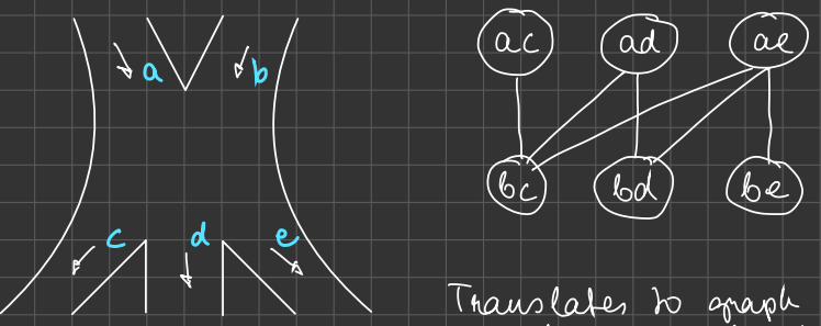
Translates to graph coloring problem and maximal independent set problem too

King Arthur and the knights of the Round Table

Noblemen and Noble Maidens

Turing Machines

definition, construction, properties, transition functions

What is a Turing Machine

• TMS are abstract models for real computers having an infinite memory
  (in the form of a tape) and a reading head
• has finite number of internal states
• has distinguished starting and final states (termination: accept / reject)
• has transition functions (Tt) (graphs)

---

• 图灵机是对真实计算机的抽象模型，它具有无限内存（以磁带的形式）和读写头
• 具有有限数量的内部状态
• 具有特殊的起始和终止状态（终止：接受/拒绝）
• 具有转换函数（Tt）（图）

---

• TM accepts the initial content of the tape if it terminates in an accepting
  state. Otherwise TM rejects it.
• TM terminates, if there is no rule with watching conditions
  for certain state and input symbols.
• TM is ND (non-deterministic), if such a state and set of input symbols
  exist, for which there are multiple rules defined.
  (= from the same set of starting state and input symbols the TM has multiple outcomes)

---

• 如果图灵机终止于接受状态，则它接受磁带的初始内容。否则拒绝。
• 如果没有匹配的规则，则图灵机终止。
• 如果存在某个状态和输入符号集，对于该状态和输入符号集，有多个规则，则图灵机是非确定性的（ND）。
  （=从同一组起始状态和输入符号集，图灵机具有多个结果）

---

• NDTM accepts the initial content of the tape if there is
  a sequence of transition functions that accepts it.

Thesis: For All NDTM Exsist equivalent DTM

对于所有的非确定性图灵机，都存在等价的确定性图灵机

Defining a Turing Machine

• defining the number of tapes & head
• defining the tape alphabets
• defining the net of state, initial and terminating states,
  accepting and rejection terminal states

From an already existing machine it is possible to head the followings:

• number of heads
• set of states constructed from the states mentioned in the TFS

Universal TM: TM, which can simulate All other TM

Church - Turing thesis:
A function (problem) can be effectively solved <=> it is computable with a TM

The same problems can be solved by a TM and modern computers

Complexity of algorithms

measuring complexity, complexity classes

算法会消耗时间和内存，复杂度就是衡量消耗的指标

时间复杂度

时间复杂度主要是循环导致的，我们不必把它想得太复杂
下面列出的时间复杂度越来越大，执行的效率越来越低

常数阶 O(1)

let i = 1;
i = i + 1;

说白了就是没有循环，即便它有几百万行

对数阶 O(logN)

let i = 1;
while (i < n) {
  i = i * 2;
}

我们可以看到，每次循环都会把 i 乘 2
设循环 x 次后，i 大于 n
则 2^x > n，即 x > log2(n)

线性阶 O(N)

for (let i = 0; i < n; i++) {
  console.log(i);
}

这个就更好理解了，循环 n 次
它的前进速度明显就没有之前乘 2 的那个快了

线性对数阶 O(NlogN)

for (let i = 1; i < n; i = i * 2) {
  for (let j = 0; j < n; j++) {
    console.log(j);
  }
}

名字看的很奇怪，但实际上
把 O(logN) 的代码，再循环 N 次
那它的时间复杂度就是 n * logn 了

当然你也可以把 O(N) 的代码，再循环 logN 次
就像上面的例子一样

平方阶 O(N^2)

for (let i = 0; i < m; i++) {
  for (let j = 0; j < n; j++) {
    console.log(j);
  }
}

n * n 不就是 n^2 吗
把 O(N) 的代码，再循环 N 次
比之前那个还好理解

当然也可以是 m * n
那时间复杂度就是 O(MN) 了

---

其他的还有

• K 次方阶 O(N^k)
• 指数阶 O(2^N)
  一般是递归算法
• O(3^N)
• etc.

计算

T(n) 算法的执行次数
T(n) = O(f(n))

1. 嵌套循环
   由内向外分析，并相乘

   // O(n)
   for (let i = 0; i < n; i++) {
     // O(n)
     for (let j = 0; j < n; j++) {
       console.log(j); // O(1)
     }
   }

   时间复杂度为 O(n * n * 1) = O(n^2)

2. 顺序执行
   你可以把它们的时间复杂度相加
   在不要求精度的情况下可以直接等于其中最大的时间复杂度

   // O(n)
   for (let i = 0; i < n; i++) {
     console.log(i);
   }
   
   // O(n^2)
   for (let i = 0; i < n; i++) {
     for (let j = 0; j < n; j++) {
       console.log(j);
     }
   }

   时间复杂度为 O(n + n^2) 或者不要求精度 O(n^2)

3. 条件分支
   时间复杂度等于所有分支中最大的时间复杂度
   说人话就是：最麻烦的那个情况

   if (n > 10) {
     // O(n)
     for (let i = 0; i < n; i++) {
       console.log(i);
     }
   } else {
     // O(1)
     console.log(n);
   }

   时间复杂度为 O(n)

空间复杂度

很显然，时间复杂度并没有真正计算算法实际的执行时间
那么空间复杂度一样也不是真正的占用空间

O(1)

let i = 1;
i = i + 1;

代码中的变量所分配的空间，都不随数据量的变化而变化
所以空间复杂度为 O(1)

O(N)

let arr = [];
for (let i = 0; i < n; i++) {
  arr.push(i);
}

看到数组就表明，空间是随着 n 增大而增大的
所以空间复杂度为 O(N)

计算

所以说的简单一点

• 如果 n 增大，程序占用的空间不变，则空间复杂度为 O(1)
• 如果 n 增大，程序占用的空间成线性增长，那么空间复杂度就是 O(N)
• 如果 n 增大，程序占用的空间成平方增长，那么空间复杂度就是 O(N^2)

以此类推
当然也有 O(N + M), O(logN)等

Sorting algorithms and their complexity

selection sort, bubble sort, insertion sort and optimization, their analysis, theorem about maximum complexity case runtime steps

我们按时间复杂度区分，并介绍十大常用的排序算法
由于这门课并不教怎么写代码，所以我们只需要了解它是怎么工作的就行了

学计算机不学写代码，行吧，当数学课上

O(N)

它们都是非比较算法，不适合大量或大范围数据

计数排序

Counting Sort
每个桶只存储单一键值
O(N + K)

对于给定的输入，统计每个元素出现的次数，然后依次把元素输出

桶排序

Bucket Sort 每个桶存储一定范围的数值
它需要调用其他的排序算法来完成排序
所以它的实际时间复杂度受到其使用的排序算法的影响
O(N * K)

基本思路是，把数据分到有限数量的桶里，然后对每个桶内部的数据进行排序
最后将各个桶内的数据依次取出，得到结果

让我们看一个例子
假设我们有 20 个数据，要分成 5 个桶

function bucketSort(arr: number[], bucketSize: number) {
  // 创建大小为 bucketSize 的桶数组
  const bucket: number[][] = [];

  // 初始化桶数组
  for (let i = 0; i < bucketSize; i++) {
    bucket[i] = [];
  }

  // 获取数组中的最大值和最小值
  const max = Math.max(...arr); // 194
  const min = Math.min(...arr); // 13

  // 计算桶的范围
  // (194 - 13 + 1) / 5 = 36.4
  const range = (max - min + 1) / bucketSize;

  // 将数据放入对应的桶中
  for (let i = 0; i < arr.length; i++) {
    // 计算数据应该放入的桶的索引
    // 比如 63：floor(63 - 13) / 36.4) = 1
    const index = Math.floor((arr[i] - min) / range);
    bucket[index].push(arr[i]);
  }

  // 使用其他算法，对桶内的数据进行排序
  for (let i = 0; i < bucketSize; i++) {
    bucket[i].sort((a, b) => a - b);
  }

  // 将桶内排好序的数据依次取出，得到有序序列
  const result: number[] = [];
  for (let i = 0; i < bucketSize; i++) {
    for (let j = 0; j < bucketSize; j++) {
      result.push(bucket[i][j]);
    }
  }

  return result;
}

基数排序

Radix Sort
根据键值的每位数字来分配桶
O(d(n+r))，其中 d 是基数，n 是要排序的数据个数，r 是每个关键字的基数

将所有待比较数值统一为同样的数位长度，数位较短的数前面补零
然后，从最低位开始，依次进行一次排序
这样从最低位排序一直到最高位排序完成以后，数列就变成一个有序序列

O(NlogN)

希尔排序

Shell Sort，也称递减增量排序
是插入排序的一种更高效的改进版本，它会优先比较距离较远的元素

先将整个序列，分割成若干个子序列，分别进行插入排序
待整个序列基本有序时，再对整体进行插入排序

---

我们有 [7, 6, 9, 3, 1, 5, 2, 4] 需要排序
首先我们确定增量为 4，每次缩小一半

所以我们有 4 个子序列

[7, 1];
[6, 5];
[9, 2];
[3, 4];

分别排序它们

[1, 7];
[5, 6];
[2, 9];
[3, 4];

得到

[1, 5, 2, 3, 7, 6, 9, 4];

然后缩小增量为 2，再次分割

[1, 2, 7, 9];
[5, 3, 6, 4];

排序得到

[1, 2, 3, 4, 5, 6, 7, 9];

归并排序

Merge Sort，是一种分治算法
将两个或两个以上的有序表合并成一个新的有序表

1. 把长度为 n 的序列分成两个长度为 n/2 的子序列
2. 对这两个子序列分别采用归并排序（递归）
3. 将两个排序好的子序列合并成一个最终的排序序列

快速排序

Quick Sort
应该算是在冒泡排序基础上的递归分治法

1. 随便选择一个元素
2. 将比这个元素小的放在左边，比这个元素大的放在右边
3. 对左右两边的元素重复第二步，直到各区间只有一个元素

堆排序

Heap Sort

1. 构建一个大顶堆，此时，整个序列的最大值就是堆顶的根节点
2. 将其与末尾元素进行交换，此时末尾就为最大值
3. 然后将剩余的 n-1 个元素重新构建成一个堆，这样会得到 n 个元素的次小值
4. 如此反复执行，便能得到一个有序序列了

O(N^2)

冒泡排序

Bubble Sort
比较相邻的元素，如果第一个比第二个大，就交换他们两个，一直向上冒泡

选择排序

Selection Sort
也就是每次找到最小的元素，放到前面，重复

优化

可以在找到最小元素时记录下它的位置，并在最后交换元素的时候使用该位置。
这样可以避免每次都将最小元素与已排序序列的最后一个元素交换，减少了不必要的操作

例如，对于序列[5, 3, 8, 1, 9]，优化的过程如下：

1. 第一次遍历，找到最小元素 1，然后将 1 与 5 交换
   [1, 3, 8, 5, 9]
2. 第三次遍历，在剩下的序列 [5, 8, 9] 中找到最小的元素 5，然后将 5 与 8 交换
   [1, 3, 5, 8, 9]

插入排序

Insertion Sort
像打扑克时整理手牌一样，将每张牌插入到合适的位置

Basic graph algorithms

graph searches (BFS, DFS, Dijsktra), tree traversals, longest path problems

深度优先搜索

广度优先搜索

遍历

前序遍历：根结点 —> 左子树 —> 右子树
是从最上层往下走

中序遍历：左子树 —> 根结点 —> 右子树
是从最左边往右走

后序遍历：左子树 —> 右子树 —> 根结点
是从最下层往上走

层次遍历：只需按层遍历即可

Dijsktra

    5
A ----- B
|       |
|       |
4       6
|       |
|       |
C ----- D
    5

首先，我们将 A 设为原点，并初始化每个顶点到原点的距离为无穷大

/**
 * 每个顶点到原点的距离
 */
let dist: Record<string, number> = {
  A: 0,
  B: Infinity,
  C: Infinity,
  D: Infinity,
};

/**
 * 获取两个顶点之间的权重
 */
declare function weight(node1: string, node2: string): number;

接下来，我们要不断迭代更新每个顶点到原点的最短距离，
直到所有顶点的最短距离，都被更新为最终值。

在每次迭代中，我们首先找到所有未被更新的顶点中，距离原点最近的顶点，
然后更新它到原点的最短距离，并根据新的距离，更新其他顶点，到原点的距离。

从 A 向外扩散

dist.B =
  Math.min(dist.B, dist.A + weight("A", "B")) =
  Math.min(Infinity, 0 + 5) =
    5;

dist.C =
  Math.min(dist.C, dist.A + weight("A", "C")) =
  Math.min(Infinity, 0 + 4) =
    4;

从 B 向外扩散

dist.D =
  Math.min(dist.D, dist.B + weight("B", "D")) =
  Math.min(Infinity, 5 + 6) =
    11;

从 C 向外扩散

dist.D = Math.min(dist.D, dist.C + weight("C", "D")) = Math.min(11, 4 + 5) = 9;

得到结果

dist = {
  A: 0,
  B: 5,
  C: 4,
  D: 9,
};

所以，从 A 到 D 的最短距离为 9

Graph diagnostics

Graph diagnostic problems are graph problems that can be answered with Y/N.

Connectivity

A graph G is connected, if for any two nodes there exists a walk between them.

---

连通性是指图中任意两个顶点之间是否存在一条路径，使得两个顶点可以互相到达。如果一个图中的任意两个顶点都可以互相到达，那么这个图就被称为连通图。

要判断一个图是否连通，可以使用搜索算法，如广度优先搜索或深度优先搜索。搜索时，从图中的任意一个顶点开始，并尝试访问该顶点的所有邻接点。如果能够访问到图中所有的顶点，那么这个图就是连通图。

Absolute winner

绝对赢家指的是一个结点，它在一个博弈论游戏中总是能够获胜。这意味着，不论对手采取什么策略，该结点都有某种优势，使它能够获胜。例如，如果一个结点具有更多的邻居，那么它就可能是一个绝对赢家，因为它可以通过与其他结点交换信息来获得更多的有利条件。

绝对赢家与相对赢家有所不同。相对赢家指的是在某些情况下，某个结点比其他结点更有优势，从而使它有可能获胜。但是，如果对手采取了特定的策略，那么这个结点可能就不再是赢家了。而绝对赢家则不存在这种情况，它总是能够获能，不管对手采取什么策略。

Complete node, logical formulas

完全节点是指，这个节点与其他任何节点都至少存在一条边

至于 logical formulas，指的是 FDNF disjunctive normal form
它与 DNF 不同点似乎是每个出现的变量都会出现在每个子句中

Graph coloring

Vertex

顶点着色的规则是，任意两个相邻的顶点不能有相同的颜色。
并且我们使用尽可能少的颜色来着色。

我们从图中的一个顶点开始，为它分配一种颜色。然后，我们按照顶点的顺序遍历图中的其他顶点，为每个顶点分配一种与相邻顶点不同的颜色

Brooks theorem

描述了图的着色数与图中最大度数的关系，提供了图着色数的一个上界

如果一个无向图 G 满足以下条件，那么它可以用 Δ(G) 或更少的颜色染色：

• G 是一个连通图（即它不包含任何脱离的部分）
• G 不包含任何奇环（即它不包含任何长度为奇数的环）
• Δ(G) 指的是图 G 中最大的度数。

Degree

度数指的是一个顶点与其相邻顶点之间的边的数量
度数可以用来衡量一个顶点与其他顶点的连通性。
通常情况下，一个顶点的度数越大，它与其他顶点的连通性就越强

Four color theorem

如果一个平面图 G 不包含任何环，那么它可以用不超过 4 种颜色染色，使得相邻的两个区域拥有不同的颜色。

Subgraph

在原图中选择一些节点和边，并从原图中删除其他的节点和边。这样得到的图就是原图的一个子图。
如果一个节点的度数为 2，那么我们可以删除该节点，并将它与其他两个节点之间的两条边”合并”成一条边。

Edge

给图中的边分配颜色，使得图中相邻的边拥有不同的颜色

Chromatic index 是图的最小着色度，指需要多少种不同的颜色

Vising theorem 指 对于任意一个无向图，它的染色度（chromatic number）不会超过其度数（degree）的上限

Bipartite graphs 是一种二分图，它由两个部分组成，每个部分内部的点互不相邻，而两个部分之间的点才会相互相邻。

Planar graphs 则是一种平面图，它是指图中任意两条边都不会相交，也就是说，图中的边可以在平面上放置而不会交叉。

---

Scheduling problems

例如，在一个工厂生产线上，有许多不同的机器和工人，他们需要按照特定的顺序来完成各种任务。为了让生产流程顺利进行，我们可以使用 edge coloring 算法来给每个任务分配一种颜色，并确保相邻的任务颜色不同。这样，工人和机器就可以按照颜色顺序来执行任务，从而保证生产流程的顺利进行。

Packing and Covering

Generalization

General, “everyday” problems, which have suboptimal solutions:

1. Put in objects into one container!
   Some pairs are incompatible, those cannot be put into the container together.
   Question: how to put the maximal number of objects into the container?

2. n people at a meeting.
   Find the largest subgroup of them, in which everybody knows everybody!

3. Trucker delivering goods with no going back
   Question: how can they deliver the maximum number of goods?

4. Big piece of leather, cutting out small shapes.
   Question: how to cut out the largest amount of smaller shapes?

Common property of these problems: representable with a graph similarly.
Is there any connection between their solutions?

Let’s look at the problems solutions, starting with the “easiest”:

---

一般来说，“日常” 问题，它们有着次优解：

1. 把物品放入一个容器中
   有些物品是不兼容的，它们不能放在同一个容器中
   问题：如何把最多的物品放入容器中？

2. n 个人在会议中
   找到其中最大的一个子集，其中每个人都认识

3. 卡车司机送货，不允许回头

4. 大块皮革，切割成小块。
   问题：如何切割出最多的小块？

这些问题的共同特点：它们可以用图来表示

Disjoint Interval Search

3. Trucker delivering goods with no going back
   Question: how can they deliver the maximum number of goods?

Disjoint Interval Search (DIS)
This problem is also called interval packing.

---

绎演丁真，鉴定为史

如果一个卡车司机要把货物送到多个不同的地方，而且一旦离开一个地方就不能再回去，
那么他应该怎样才能把尽可能多的货物送到目的地呢？

我寻思着这问题应该用 TSP 来解才对
总之先看看什么是 DIS

DIS 是一种用于处理区间数据的算法。
区间数据是指一组由起始和结束点表示的区间，例如：[1, 5]、[10, 15] 等。
它能够快速检索出与给定的区间不相交的区间。

1. 将区间数据存储在能够快速查找和插入的数据结构中，例如红黑树、平衡树或 B 树
2. 查找与给定区间不相交的区间
   检查区间数据中的每一个区间，并判断它们是否与给定区间不相交
   如果一个区间与给定区间不相交，则将其加入结果集。
3. 返回结果集

Clique

n people at a meeting.
Find the largest subgroup of them, in which everybody knows everybody!

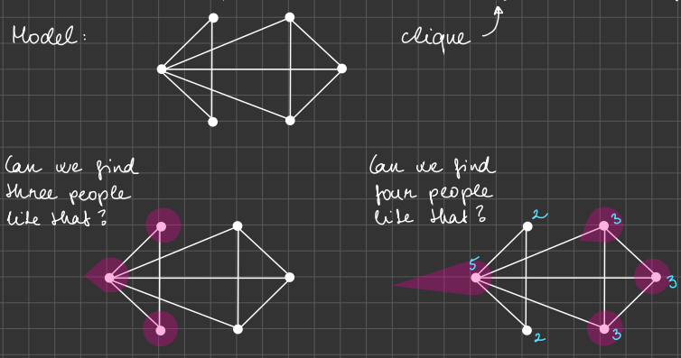
Can we find three people like that?
Can we find four people like that?
Can we find five people like that? Why not?
Clique search

---

衣掩丁真，鉴定为衣驼使

这是一个分团问题
Clique search 是一种用于寻找图中的完全子图（即“clique”）的算法
完全子图是指一个子图中所有节点都相互连通
算法需要枚举所有可能的完全子图，并确定哪些子图满足给定的条件

Maximal Independent Set

Put in objects into one container!
Some pairs are incompatible, those cannot be put into the container together.
Question: how to put the maximal number of objects into the container?

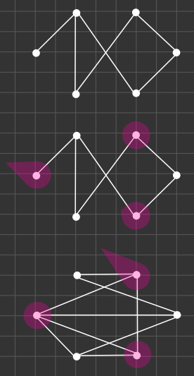
Edges code incompatibility.
We are searching for independent node subsets.
Maximal Independent Set (MIS)

We found a maximal empty subgraph.

Connection with the previous problem?
If we create the complimenting graph from this (where we had an edge, now we don’t have one, and vice versa), and consider the same chosen nodes, then that is a clique.

So we can convert this problem into the previous one: MIS → Clique search

These problems are basically the same, only their representation is different.

In this sense, even problem no.3 is the same as no.1 and no.2.

Converting problem no. 3 to the present form:

Intervals are going to turn into vertices of a graph.
If two intervals are incompatible, we draw an edge between the corresponding nodes.

We converted DIS into MIS.

---

Maximal Independent Set 是指一个图中没有一个节点与其他节点相邻，
并且该集合不能再增加任何节点而保持这种性质的节点集合

一个独立集（也称为稳定集）是一个图中一些两两不相邻的顶点所形成的集合，
如果两个点没有公共边，那么这两个点可以被放到一个独立集中

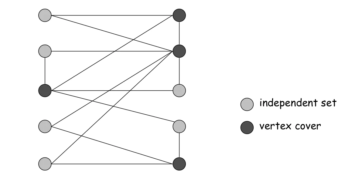
对于三个点组成的完全图而言，每个点自身是一个独立集（且是最大独立集）
对四个点构成的四边形图而言，对角的两个点组成一个独立集（且是最大独立集）

如果往图 G 的独立集 S 中添加任一个顶点都会使独立性丧失（亦即造成某两点间有边），那么称 S 是极大独立集。

如果 S 是图中所有独立集之中基数最大的，那么称 S 是最大独立集，且将该基数称为 G 的独立数，记为 α(G)。一般来讲，图 G 中可能存在多个极大独立集和最大独立集。

根据定义，最大独立集一定是极大独立集，但反之未必。

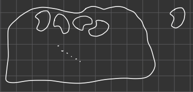
Cut

Big piece of leather, cutting out small shapes.
Question: how to cut out the largest amount of smaller shapes?

大块的皮革，切出小的形状。
问：如何切出最多的小形状？

We can rotate the sample, but we still have to fit into the big piece of leather.

我们可以旋转样本，但我们仍然要贴合大块皮革。

This is the most difficult problem out of the four, because the main “philosophical” difference between them is that the first three were obvious finite problems (finite number of people, objects, intervals), whereas this problem cannot produce obvious finite number of nodes.

这是四个问题中最困难的一个，因为它们之间的主要“哲学”区别在于前三个是显然的有限问题（人数、物品数、区间数都是有限的），而这个问题不能产生显然的有限节点数。

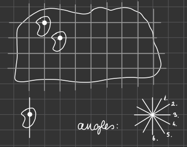
So we make a grid on the big leather, place a node on the shape, and say that the shape can only be cut out of that node fits on one of the grid points.

因此，我们在大皮革上做一个网格，在形状上放一个节点，并说形状只能在该节点适合网格点之一时被切出来。

The grid points create a finite set. But since we can still rotate the shape around the grid point, our choices are infinite again. Solution: we only consider a few angles. So now we can only cut out the shape if the node is ou a grid point, and the line on the sample can only parallel to one of our predefined angle lines.

网格点创建了一个有限集。但是，由于我们仍然可以围绕网格点旋转形状，所以我们的选择又是无限的。解决方案：我们只考虑几个角度。因此，现在我们只能在节点在网格点上并且样本上的线只能与我们预定义的角度线平行时切出形状。

So to make an infinite problem finite we need to add restrictions.

因此，要使无限问题变为有限，我们需要增加限制。

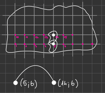
We can code the placement with the number of the grid point and the number of the angle.
Eg: (5; 6) and (14; 6).

我们可以用网格点的编号和角度的编号来编码放置位置。例如：（5；6）和（14；6）。

However, these two overlap, so they cannot be cut out together. This incompatibility can be represented in a graph by adding an edge between these two number pains.

然而，这两个重叠了，因此它们不能一起切出来。这种不兼容可以通过在这两个数字之间添加一条边来表示在图中。

This way we can create a graph, and the maximum number of cutouts on the leather is reduced to finding the maximal number of independent nodes in the corresponding graph.

这样我们就可以创建一个图，皮革上的最大切割次数就被减少到在相应图中找到最大的独立节点数。

What is the problem with this method?
The restrictions can cause a result with less cutouts, than if we could freely place the shape.

这种方法有什么问题？
限制可能导致切割次数比我们可以自由放置形状时少的结果。

Solution: let’s use a denser grid and consider none rotational angles!

解决方案：让我们使用更密集的网格并考虑非旋转角度！

Problem with the solution: as we have more gridpoints and angles, the graph becomes larger, so finding the MI5 is more complicated.

解决方案的问题：随着我们有更多的网格点和角度，图变得更大，因此找到 MI5 变得更复杂。

So this method is a digitalization, which has a resolution. The bigger the resolution is, the closer to the optimal solution we are.

因此，这种方法是一种数字化，它具有分辨率。分辨率越大，我们越接近最优解。

总结

Ater examining these four problems, we have a general framework:

在经过对这四个问题的检查后，我们得出了一个总体框架：

Given is a graph. Find the maximal number of nodes such that those are never connected to each other. <=> We want to find the maximal independent set of nodes. → MIS problem.

给定一张图。找到一个节点的最大数量，这些节点从不相互连接。<=>我们想找到节点的最大独立集合。→MIS 问题。

This can be solved in exponential time.

这可以在指数时间内解决。

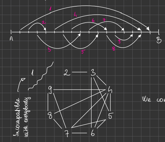
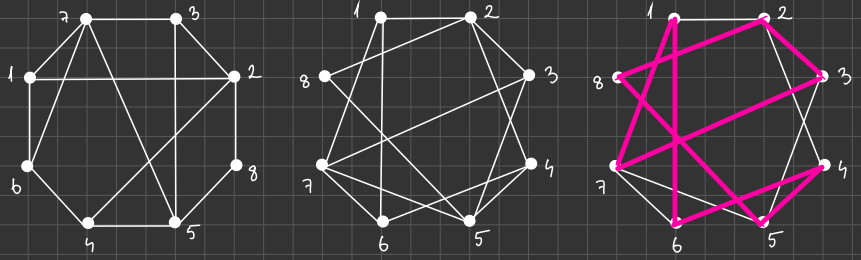
The trivial algorithm for finding MIS:

找到 MIS 的简单算法：

We want to find MIS of { 1, 2, 3, 4, 5, 6 }. We try to find an independent subset of size 2. Start with 41,2}. Is this independent? No! So try { 1, 3 }. This is good! But then can we find an independent subset of nite 3? We need to check all site 3 subsets.

我们想找到 {1,2,3,4,5,6} 的 MIS。我们试图找到大小为 2 的独立子集。从 {1,2} 开始。这是独立的吗？不是！所以尝试 {1,3}。这很好！但是然后我们能找到大小为 3 的独立子集吗？我们需要检查所有大小为 3 的子集。

In the worst case we need to investigate all subsets of { 1, 2, 3, 4, 5, 6 }

在最坏的情况下，我们需要调查 {1,2,3,4,5,6} 的所有子集

Theorem: If |x| = n, then |p(x)| = 2^n.

(p(x) = { y | y <= x } -> power set = set of all subsets)

In our example n = 6, so we have 2^6 = 64 subsets.

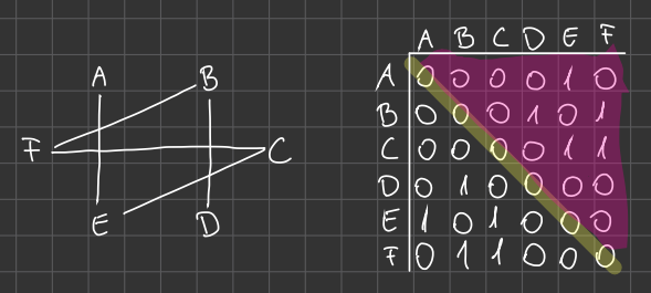
How to code subsets?

{ 1, 2, 3, 4, 5, 6 }

1	0	1	0	0	0
1	1	0	0	0	1

-> this will code { 1; 3 }
-> this will code { 1; 2; 6 }

Since it is a one-to-one correspondence between subsets and outshines,
then |p(x)| = |{ binary string of length 8 }|

因为子集和出现之间是一一对应的，所以 |p(x)| = |{长度为 8 的二进制字符串}|

because a choice codes 1 On 0 = yes or no

因为选择编码 1 On 0 = yes or no

In terms of our MIS - finding problem: if we count checking a binary string for independence, then this trivial algorithm has an exponential runtime, exactly 2^n.

就我们的 MIS 查找问题而言：如果我们算出检查一个二进制字符串是否独立的次数，那么这个简单算法的运行时间是指数级别的，精确地说是 2^n。

A more refined algorithm for the same problem:
Find a method, where we only check already independent sets.

同一问题的一种更优秀的算法：
找到一种方法，只检查已经独立的集合。

Example:

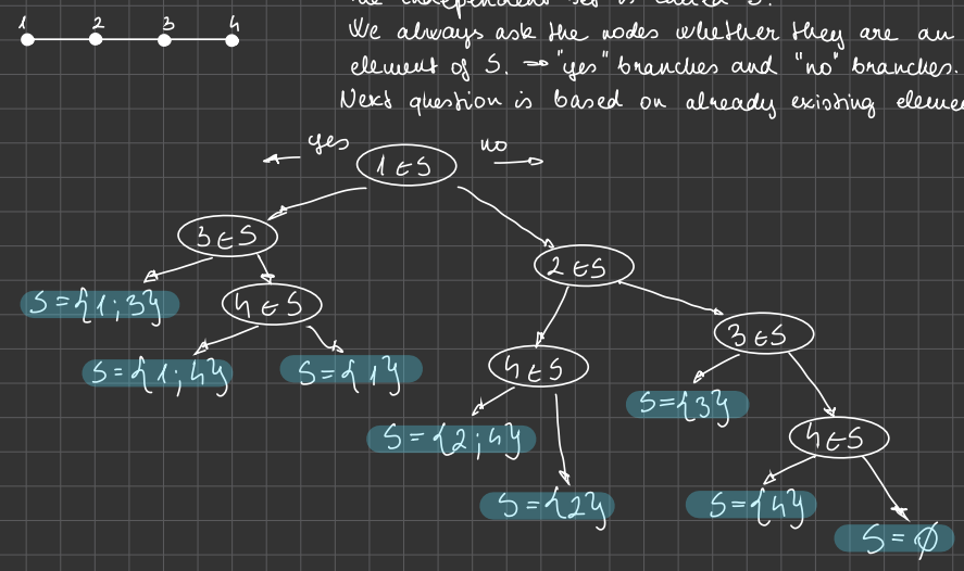
The independent set is called S.
We always ask the nodes whether they are an element of S. → “yes” branches and “no” branches. Next question is based on already existing elements.

独立集合称为 S。
我们总是问节点是否是 S 的元素。→“是”和“否”分支。下一个问题是基于已存在的元素。

This is a labelled and rooted binary thee.
Can be done faster, if we are only considering paths that have a chance to have enough nodes on them.
“if it’s not there, don’t even look”

这是一棵带标签和根的二叉树。
如果我们只考虑可能有足够节点的路径，可以更快地完成。
“如果它不在那里，甚至都不用看”。

Interval packing, dominating sets

A little help for the next algorithm: the Pidgeon-hole principle.

下一算法的一点帮助：鸽巢原理。

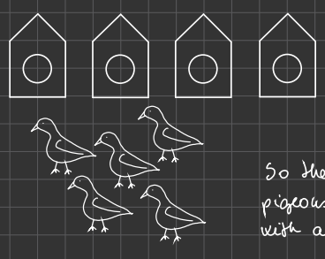
Question: when the pigeons go to their pigeon-holes, what can we state for sure?
Whichever houses they choose, there is going to be at least one hole with two pigeons in it.

问题：当鸽子去它们的鸽巢时，我们能肯定什么？
无论它们选择哪所房子，至少会有一个洞有两只鸽子。

So the pigeon-hole principle says that if there are more pigeons than houses, then there will be at least one hole with at least two pigeons in it.

因此，鸽巢原理说，如果有比房子更多的鸽子，那么至少会有一个洞至少有两只鸽子。

If this weren’t true, and all houses tould contain one pigeon at worst, then there would be only as many pigeons as houses. Whereas we had more pigeons.

如果这不是真的，并且所有的房子里最多只有一只鸽子，那么只会有和房子一样多的鸽子。但我们有更多的鸽子。

If we use our previous example 3, we can apply the pigeon-hole principle to the problem:

如果我们用之前的例子 3，我们可以将鸽巢原理应用于问题：

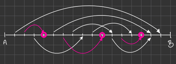
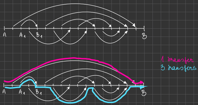
The algorithm: choose closest destination, if starting point is still ahead
=> maximal number of => independent intervals => Interval packing algorithm

算法：如果起点仍然在前面，则选择最近的目的地
=>最大数量的=>独立区间=>区间打包算法

If we only consider the destinations as pink dots, then we can choose any interval, there will always be a pink dot on it - at least one dot.
=> the set of pink dots is a dominating set.

如果我们只考虑目的地作为粉红色点，那么我们可以选择任何区间，它上面总会有一个粉点——至少有一个点。
=>粉点集是一个支配集。

A set X is a dominating set, if for every you find at least one element of the set on that interval.

一个集合 X 是支配集，如果对于每个区间都能找到集合中的至少一个元素。

Femina: X is a dominating set, 4 is an independent set of intervals.
Then |x| >= |y|.

X 是支配集，4 是区间的独立集。

The chosen intervals corresponding to the transportation is an independent set with three intervals. There are also three pink dots as the dominant set. So based on the lemma, there can be no more independent intervals.

选择的区间对应于运输是具有三个区间的独立集。还有三个粉红色的点作为支配集。因此，根据引理，不能有更多的独立区间。

Proof: Indirectly. New statement: |x|birds < |y|houses.

Let’s have one more independent interval. But according to the pigeon-hole principle, there is at least one pint dominating dot on every interval. In order to dominate the all intervals, we would need at 1 different pink dots.

让我们再来一个独立区间。但根据鸽巢原理，每个区间都至少有一个主要点。为了控制所有区间，我们需要至少 1 个不同的粉点。

=> There must be at least two intervals with the same pink dot,but then they’re not independent.

=> 必须有至少两个区间有相同的粉点，但这样它们就不是独立的了。

Even though there is no general quick (polynomial) solution for
finding MIS, the Interval pairing algorithm is fast. How fast?

尽管没有求解 MIS 的通用快速（多项式）解决方案，但 Interval pairing 算法是快速的。它有多快？

We shone all starting and destination point somehow - e.g. by numbers.
So we only have to order them, and find the “smallest” endpoint first.

我们用某种方式给所有起点和终点标号——例如，用数字。
所以我们只需要按顺序排序，找到“最小”的终点。

~n steps needed to find the closest destination
we need to repeat it at worst a times => polynomial algorithm

找到最近目的地需要 ~n 步
最坏情况下，我们需要重复 a 次，所以这是一个多项式算法

How can it be that MI5 can’t be solved quickly, but this algorithm has quadratic runtime?!

为什么 MI5 无法快速解决，但这个算法的运行时间是二次的呢？

The intervals are represented as nodes and overlaps as edges in the graph.
So did we just solve MI5 in quadratic time?!

区间在图中表示为节点，重叠部分表示为边。
所以我们刚刚在二次时间内解决了 MI5 吗？

No! Because not all graphs can be processed by this method. (Not all graphs with a nodes occur this way.) so we only solved MI5 for a subset of graphs having a nodes.

不是的！因为并不是所有图都可以用这种方法处理。（不是所有带有 n 个节点的图都是这样出现的。）所以我们只为一个带有 n 个节点的图子集解决了 MI5。

So for a subset of cases we have a solution, but not for the general case.
(e.g. 5th degree polynomials)

所以对于一个子集的情况，我们有一个解决方案，但不是通用情况。（例如，五次多项式）

---

区间打包，用于找到最多可以放在一个容器内的不相交区间的最大数量。是指把一系列区间尽可能多地放到一个集合中，使得它们都不重叠。

支配集指在一张图中，存在一组节点，每个节点都与它相邻的节点相连，或者至少有一个节点在该组中。其中的元素可以覆盖整个集合，即每个元素都与至少一个其他元素有交集。

Suboptimal algorithms

次优算法

what is the basic problem?
→ polynomial algorithms are “quick”
→ exponential algorithms are “very slow”

基本问题是什么？
→ 多项式算法“快”
→ 指数算法“非常慢”

There is a set of problems for which there is no quick algorithm.

有一类问题没有快速算法。

Their runtime is proportionate to f(a) =2^n. To put this in perspective, there are no more than 2^350 atoms in the whole universe.

它们的运行时间与 f(a) = 2^n 成比例。
为了更好地理解这一点，整个宇宙中没有超过 2^350 种原子。

Therefore we can just use this disadvantage to our advantage by using these kind of problems for coding protocols, as decoding them would tale over a million years.

因此，我们可以利用这个缺点，通过使用这类问题来编写编码协议，因为解码它们需要超过一百万年。

Good example for this is finding a Hamiltonian cycle in a graph. Creating is easy, but then we can obfuscate it.

寻找图中的汉密尔顿回路是一个很好的例子。
创建容易，但是我们可以混淆它。

Problem is, that there are a lot of real-life situations that can only be converted into these kinds of problems, where the solution is exponential, or even worse.

问题是，有很多现实生活中的情况只能转换为这类问题，其解是指数级的，甚至更糟。

Good example is the traveling agent problem. This is understood on weighed graphs, and the point is to touch all the nodes with a minimal sum of edge weights. (Hamiltonian path problem).

一个很好的例子是旅行代理问题。这在加权图上是可以理解的，其目的是以最小的边权和触摸所有节点。（汉密尔顿路径问题）

In this case we can imagine a package delivery service, in which case we need the shortest possible combination / permutation of the packages in order to make the least amount of kilometers. Though, this is a hard problem, meaning, there exists not a quick algorithm for this.

在这种情况下，我们可以想象一个包裹配送服务，在这种情况下，我们需要包裹的最短可能组合/排列，以便减少尽可能多的公里数。尽管这是一个难题，即不存在一个快速的算法来解决这个问题。

=> suboptimal algorithms
-> We don’t want to (= can’t) find the best solution, but something that is pretty close this best solution.

=> 次优算法
-> 我们不想（也不能）找到最优解，而是找到一个非常接近最优解的解决方案。

So in case of the traveling agent, we don’t want to find the optimal route, but we want a route such that it is sure that it uses at more Klia as many kilometers as the optimal one. It would be a 2-optimal algorithm.

所以在旅行代理的情况下，我们不想找到最优路线，而是想找到一条路线，使得它确保它使用的公里数至少与最优路线相同。这将是一个 2-optimal 算法。

So the suboptimality of algorithms has nothing to do with running time.

因此，算法的次优性与运行时间无关。

In the traveling agent situation a 3-optimal algorithm would find a solution that is at most three times worse than the optimal one, meaning, it would find a permutation of the target adnesses such that if the driver follows that order, than at most three times as many kilometers are used as in case of the optimal solution.

在旅行代理的情况下，3-optimal 算法将找到一个至多比最优解差三倍的解决方案，这意味着它会找到目标地址的一个排列，如果司机遵循这种顺序，那么至多会使用三倍于最优解情况下的公里数。

An algorithm is called k-optimal (k ≥ 1) if its output is at most b-times worse than the best output would be.

如果其输出最多比最佳输出差 b 倍，则称该算法为 k-optimal（k ≥ 1）。

Bin packing problem

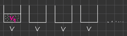
Objects with volumes:
V1, V2, V3 … Vn.

Vi <= (i = 1, …, n)

Problem: use the least amount of containers to store all objects.

问题：使用最少的容器来存储所有物品。

(The sum of the volumes of objects in one container can’t exceed volume of the container.)

（一个容器中物品的总体积不能超过容器的体积。）

This is a hard problem. But there exists a 2-optimal algorithm for that.

这是一个难题。但是存在一个 2-optimal 算法。

First Fit Algorithm: Choose the first container in which the object fits. (This is greedy.)

首次适应算法：选择第一个容器，其中的物品适合。（这是贪婪的。）

降序首次适应算法

First Fit Decreasing

1. 将物品按照价值从大到小排序
2. 找到一个能放下物品的背包，放入物品
3. 重复 2，直到所有物品都放入

简而言之，FFD 按照大小降序排列项目，然后放入第一合适的背包

Algebraic algorithms

Divisibility, Euclidean algorithm

Faster multiplication and division of large numbers